Project 02: Car Crash Exploratory Data Analysis

This project uses exploratory data analysis to visualize underlying car crash data for Southeast Michigan. This step uses python, pandas, matplotlib, and seaborn to highlight trends that exist within the data.

import pandas as pd

df = pd.read_csv('combined_dataset.csv')
#df = pd.read_csv('crash_funding_data.csv')

/Users/connorlockman/anaconda3/lib/python3.7/site-packages/IPython/core/interactiveshell.py:3057: DtypeWarning: Columns (28,48,49) have mixed types. Specify dtype option on import or set low_memory=False.
  interactivity=interactivity, compiler=compiler, result=result)

df.head()

	Unnamed: 0	ACOUNT	ALCOHOL	BCOUNT	BICYCLE	CARTODB_ID	CCOUNT	CNTNAME	COMMERCIAL	COMMUNITY	...	UNITS	WEATHER	WEEKDAY	WORK_ZONE	X	XCORD	Y	YCORD	YEAR	YOUNG
0	0	0	0	0	0	NaN	0	Washtenaw	NaN	Ann Arbor	...	2	5	2	NaN	-83.771023	-83.77102	42.287878	42.28787	2017	0
1	1	0	0	0	0	NaN	0	Oakland	NaN	Brandon Twp	...	1	5	2	NaN	-83.421944	-83.42194	42.810271	42.81026	2017	1
2	2	0	0	0	0	NaN	0	Oakland	NaN	Bloomfield Twp	...	1	5	2	NaN	-83.234323	-83.23432	42.615461	42.61546	2017	1
3	3	0	0	0	0	NaN	0	Oakland	NaN	Orchard Lake Village	...	2	2	3	NaN	-83.362812	-83.36281	42.578827	42.57882	2017	0
4	4	0	0	0	0	NaN	0	Livingston	NaN	Hartland Twp	...	2	2	5	NaN	-83.753034	-83.75303	42.656270	42.65626	2017	0

5 rows × 61 columns

What does our combined dataset look like?

len(df)

709900

We have 709,900 crash cases in this dataset.

what about the distribution among years?

import numpy as np
import pandas as pd
import seaborn as sns
import matplotlib.pyplot as plt
from scipy import stats
sns.set(color_codes=True)

x = df['YEAR']

yr_2014 = len(df.loc[df['YEAR'] == 2014])
yr_2015 = len(df.loc[df['YEAR'] == 2015])
yr_2016 = len(df.loc[df['YEAR'] == 2016])
yr_2017 = len(df.loc[df['YEAR'] == 2017])
yr_2018 = len(df.loc[df['YEAR'] == 2018])

yr_2017

145362

x_axis = ['2014','2015','2016','2017','2018']

y_axis = [yr_2014,yr_2015,yr_2016,yr_2017,yr_2018]

sns.barplot(x=x_axis, y=y_axis)

<matplotlib.axes._subplots.AxesSubplot at 0x10a7701d0>

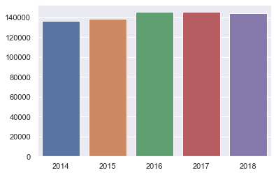
We see that each year has a very similar total number of car crashes.

When are these car crashes occuring?

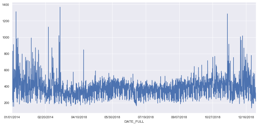
Let’s look at the aggregate day counts

dates_result = df.groupby('DATE_FULL').size().sort_values(ascending=True)

dates_result

DATE_FULL
12/25/2014     136
01/01/2015     155
01/03/2016     155
12/25/2015     156
03/23/2014     160
07/06/2014     162
03/30/2014     163
12/25/2016     169
04/13/2014     172
07/05/2015     174
04/27/2014     176
04/05/2015     181
04/20/2014     183
04/06/2014     185
01/12/2014     185
09/09/2018     186
03/04/2018     186
02/25/2018     188
03/11/2018     188
12/07/2014     188
03/16/2014     189
03/29/2015     190
12/28/2014     191
02/19/2017     191
12/27/2015     192
11/26/2015     192
12/25/2018     193
07/16/2017     193
12/14/2014     193
04/22/2018     194
              ...
10/31/2014     768
11/20/2018     778
12/24/2017     780
12/11/2016     794
01/10/2017     795
12/18/2015     796
02/09/2018     797
01/16/2014     797
01/31/2017     818
01/02/2014     832
02/09/2016     845
04/17/2018     848
12/13/2017     870
03/01/2016     872
02/05/2014     874
01/09/2015     879
01/03/2014     913
11/21/2015     917
03/13/2014     941
12/09/2017     965
01/08/2014     982
01/09/2018     992
01/29/2018     993
12/08/2016    1007
12/11/2017    1018
03/12/2014    1021
02/24/2016    1126
11/19/2014    1287
01/07/2014    1313
03/13/2017    1369
Length: 1826, dtype: int64

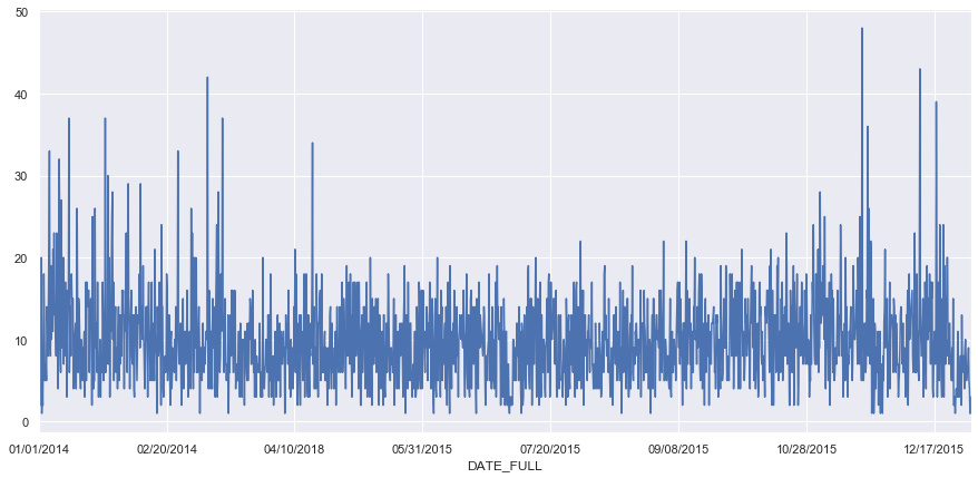
We see that the most car crashes in this dataset occurred on March 13th of 2017. With a little investigation we see that the bottom of the list makes sense with christmas day emerging as one the days with the least number of car crashes. Days at the top of this list mainly fall in the winter months and we can see that with some investigation that these days typically had wintery conditions with snow, ice, or very low temperatures occuring.

fig, ax = plt.subplots(figsize=(15,7))
result_dates = df.groupby('DATE_FULL').size().plot(ax=ax)

Let’s look at the hourly distribution of crashes

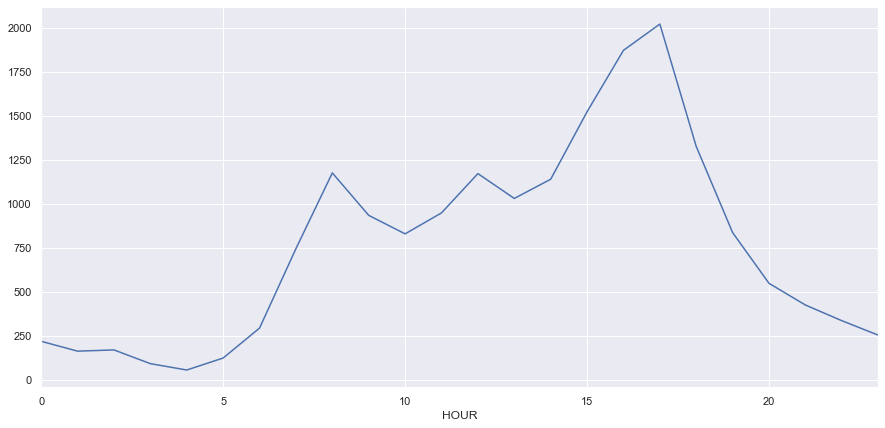
fig, ax = plt.subplots(figsize=(15,7))
df.groupby('HOUR').size().plot(ax=ax)

<matplotlib.axes._subplots.AxesSubplot at 0x116c99b38>

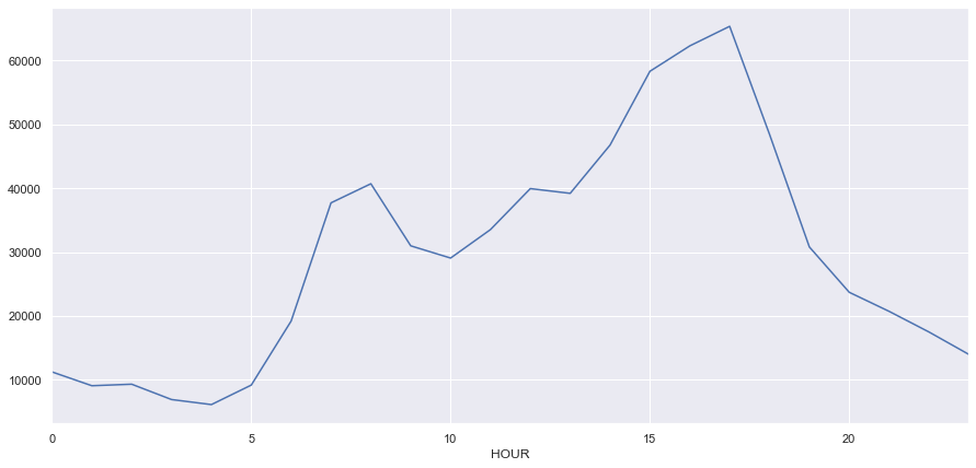
We can see in this figure that their is a bimodial distribution of crashes with a spike in the morning during the traditional morning rush hour times of 6 - 9 and a larger spike in the afternoon around 5 - 7 pm during the evening rush hour period. Intuitively, this makes sense.

Which city has the most car crashes and the least?

df.groupby('COMMUNITY').size().sort_values(ascending =True)

COMMUNITY
Novi Twp                              1
Southfield Twp                        1
Fenton (Livingston)                   1
Estral Beach                          5
Grosse Pointe Shores (Macomb)        11
Lake Angelus                         14
Leonard                              17
Memphis (St. Clair)                  17
Barton Hills                         21
Petersburg                           22
Maybee                               29
Emmett                               39
Richmond (St. Clair)                 39
Memphis (Macomb)                     44
Armada                               61
Luna Pier                            76
Carleton                             89
Yale                                 98
Algonac                             124
Capac                               128
Freedom Twp                         140
Milan (Monroe)                      143
East China Twp                      153
Manchester                          154
Ortonville                          170
Grosse Pointe Shores (Wayne)        176
Pinckney                            199
South Rockwood                      199
River Rouge                         218
Grant Twp                           218
                                  ...  
Redford Twp                        6079
Dearborn Heights                   6163
Ypsilanti Twp                      6341
Pittsfield Twp                     6852
St. Clair Shores                   7470
Madison Heights                    7511
West Bloomfield Twp                7684
Bloomfield Twp                     7948
Westland                           8590
Waterford Twp                      9357
Shelby Twp                         9407
Macomb Twp                         9426
Roseville                          9626
Novi                              10128
Pontiac                           10160
Auburn Hills                      10435
Royal Oak                         10582
Canton Twp                        10609
Taylor                            11847
Clinton Twp                       11957
Rochester Hills                   11959
Farmington Hills                  15760
Troy                              17085
Dearborn                          17505
Southfield                        18002
Ann Arbor                         18250
Livonia                           18341
Warren                            23681
Sterling Heights                  23796
Detroit                          115539
Length: 237, dtype: int64

237 cities featured crash data for the region

We see that Detroit emerges as the city with the most crashes. We can believe this because it is clearly the largest city in South East Michigan with a population close to 675,000. It is also the economic center of the region and has many of the areas jobs. Cities that fall to the bottom of the list have, generally smaller populations. For insantance, Barton Hills which is located just to the west of ann arbor had 21 crashes and has a population of 320. These results pose a question of how to normalize this data and whether that should be by total population or number of jobs in the region. We decide to rely on the raw data because we don’t have an indication about which is the appropriate normalization process.

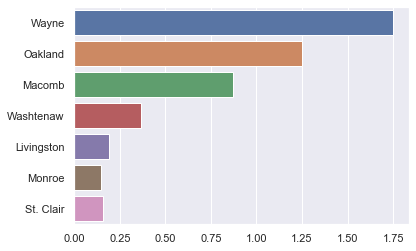
County

df.groupby('CNTNAME').size().sort_values(ascending =False)

CNTNAME
Wayne         260891
Oakland       204977
Macomb        125741
Washtenaw      56091
Livingston     24111
Monroe         19052
St. Clair      19037
dtype: int64

pop = [1.75,1.25,.871,.368,.189,.149,.159]
county = ['Wayne','Oakland','Macomb','Washtenaw','Livingston','Monroe','St. Clair']

sns.barplot(x=pop, y=county)

<matplotlib.axes._subplots.AxesSubplot at 0x1162a79b0>

Who is involved in these car crashes?

who_df = df[['PEDESTRIAN', 'BICYCLE', 'MOTORCYCLE',
       'TRAIN', 'DISTRACTED','ELDERLY','YOUNG']]

who_df.head()

	PEDESTRIAN	BICYCLE	MOTORCYCLE	TRAIN	DISTRACTED	ELDERLY	YOUNG
0	0	0	0	0	0	0	0
1	0	0	0	0	0	0	1
2	0	0	0	0	1	0	1
3	0	0	0	0	0	0	0
4	0	0	0	0	0	0	0

ped_lst = df.loc[who_df['PEDESTRIAN']==1]

ped = len(ped_lst)

ped / 709000

0.008899858956276445

bike_lst = df.loc[who_df['BICYCLE']==1]

bike = len(bike_lst)

moto_lst = df.loc[df['MOTORCYCLE']==1]

moto = len(moto_lst)

train_lst = df.loc[df['TRAIN']==1]

train = len(train_lst)

distracted_lst = df.loc[df['DISTRACTED']==1]

distracted = len(distracted_lst)

young_lst = df.loc[df['YOUNG']==1]

young = len(young_lst)

young / 709000

0.3330253878702398

old_lst = df.loc[df['ELDERLY']==1]

old = len(old_lst)

x_axis = ['ped','bike','moto','train']
y_axis = [ped, bike,moto,train]

sns.barplot(x=x_axis, y=y_axis)

<matplotlib.axes._subplots.AxesSubplot at 0x1181a75f8>

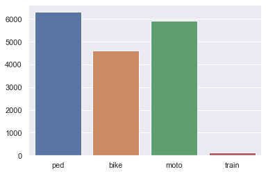
We can see here that pedestrians are involved in the most crash instances while trains are fairly rare in the crash data.

x_axis = ['old','young','distracted']
y_axis = [old, young,distracted]

sns.barplot(x=x_axis, y=y_axis)

<matplotlib.axes._subplots.AxesSubplot at 0x119e3c0b8>

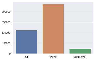
old + young + distracted

372701

709900 - 372701

337199

We see that with using some of the demographic features that we are still 337,199 crash accounts short. This builds insight into that while we do know a little about who is involved in these crashes, we don’t have full understanding about them across the board.

Weather

How does weathe impact this car crash data?

df.groupby('WEATHER').size().sort_values(ascending =False)

WEATHER
1     436696
2     142019
4      63503
5      47649
98     11278
3       3289
7       2354
8       2000
6       1019
9         42
10        27
0         24
dtype: int64

1 = clear

2 = cloudy

3 = FOG

4 = RAIN

5 = SNOW

6 = SEVERE CROSSWINDS

7 = SLEET / HAIL

8 = BLOWING SNOW

9 = BLOWING SAND SOIL DIRT

10 = SMOKE

98 = UNKNOWN

0 = NOT ENTERED

Y = [436696,142019,63503,47649,11278,3289,2354,2000,1019,42,27,24]
#X = [1,2,4,5,98,3,7,8,6,9,10,0]
X = ['CLEAR','CLOUDY','FOG','RAIN','SNOW','SEVERE CROSSWINDS','SLEET / HAIL','BLOWING SNOW','BLOWING SAND SOIL DIRT','SMOKE','UNKNOWN','NOT ENTERED']

sum(Y)

709900

Every case in the data has a weather code assigned to it.

sns.barplot(x=X, y=Y)
plt.xticks(rotation='vertical')

(array([ 0,  1,  2,  3,  4,  5,  6,  7,  8,  9, 10, 11]),
 <a list of 12 Text xticklabel objects>)

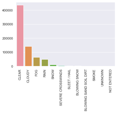
The vast majority of crashes occur under clear or cloudy circumstances.

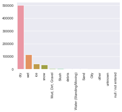
Road Conditions

Weather doesn’t seem to be a major factor, but could road factors be impacting the data?

df.columns

Index(['Unnamed: 0', 'ACOUNT', 'ALCOHOL', 'BCOUNT', 'BICYCLE', 'CARTODB_ID',
       'CCOUNT', 'CNTNAME', 'COMMERCIAL', 'COMMUNITY', 'CRASHID', 'CRSHTYPEO',
       'DATE_FULL', 'DAY', 'DEER', 'DISTRACTED', 'DIS_CTRL_I', 'DRUG',
       'ELDERLY', 'EMERGENCY', 'FALINKID', 'FID', 'HIGH_SEVER', 'HITNRUN',
       'HOUR', 'HWY_CLSS_C', 'INTERROAD', 'INTR_INVL_', 'JURIS', 'KCOUNT',
       'LANEDEPART', 'LIGHTING', 'MAINROAD', 'MONTH', 'MOTORCYCLE', 'MP',
       'NFC', 'OBJECTID', 'OCCUPANTS', 'PEDESTRIAN', 'PR', 'PROPDAMG',
       'REDLIGHTRU', 'ROADCONDIT', 'ROADLANES', 'SCHOOLBUS', 'SEMMCD',
       'SPEEDLIMIT', 'SURFACE', 'TIME_FULL', 'TRAIN', 'UNITS', 'WEATHER',
       'WEEKDAY', 'WORK_ZONE', 'X', 'XCORD', 'Y', 'YCORD', 'YEAR', 'YOUNG'],
      dtype='object')

df.groupby('WORK_ZONE').size().sort_values(ascending =False)

WORK_ZONE
0.0    141201
1.0      2743
dtype: int64

2743 + 141201

143944

We can’t be certain of anything about workzones because it appears that we dont have data for many of the years in question

df.groupby('ROADCONDIT').size().sort_values(ascending =False)

ROADCONDIT
1     500506
2     114178
4      41835
3      34048
6       6193
98      4955
97      3390
8       2250
5       2185
7        254
10        47
0         38
9         21
dtype: int64

1 = dry

2 = wet

3 = ice

4 = snow

5 = Mud, Dirt, Gravel

6 = slush

7 = debris

8 = Water (Standing/Moving)

9 = Sand

10 = Oily

97 = other

98 = unknown

0 = null / not entered

Y = [500506,114178,41835,34048,6193,4955,3390,2250,2185,254,47,38,21]
X = ['dry','wet','ice','snow','Mud, Dirt, Gravel', 'Slush','debris','Water (Standing/Moving)','Sand','Oily','other','unknown','null / not entered']

sns.barplot(x=X, y=Y)
plt.xticks(rotation='vertical')

(array([ 0,  1,  2,  3,  4,  5,  6,  7,  8,  9, 10, 11, 12]),
 <a list of 13 Text xticklabel objects>)

df.groupby('HWY_CLSS_C').size().sort_values(ascending =False)

HWY_CLSS_C
9    420484
3    129568
1    103871
2     41057
4      9031
5      4076
7      1079
0       734
dtype: int64

df.groupby('ROADLANES').size().sort_values(ascending =False)

ROADLANES
 2    252048
 5    134424
 3    132193
 4    125930
 1     24694
 6     23295
 7     12496
 8      4144
 9       632
 0        40
-2         2
-4         2
dtype: int64

df.groupby('SPEEDLIMIT').size().sort_values(ascending =False)

SPEEDLIMIT
45    160483
25    114022
35     95293
70     86459
40     82383
55     73438
50     49487
30     33187
0       8746
15      2520
60      1406
20       923
65       781
10       355
5        216
75       195
46         2
26         1
23         1
8          1
80         1
dtype: int64

df.groupby('SURFACE').size().sort_values(ascending =False)

SURFACE
Asphalt     91780
Concrete    39784
            10760
Gravel       1609
Brick          11
dtype: int64

Road Funding

We are interested in building road funding into this data and conducting some analysis on this

df_funding = pd.read_csv('community.csv')

df_funding.head()

	County	Community	Annual Amount	Road Miles	Average Per Mile	Unnamed: 5	Unnamed: 6
0	Livingston	Brighton	$465,346	29.44	$15,807	NaN	NaN
1	Livingston	Fowlerville	$207,751	13.84	$15,011	NaN	NaN
2	Livingston	Howell	$576,420	36.64	$15,732	NaN	NaN
3	Livingston	Pinckney	$150,719	11.37	$13,256	NaN	NaN
4	Macomb	Armada	$106,664	7.21	$14,794	NaN	NaN

df_funding = df_funding.rename(columns={'Community': 'COMMUNITY'})

df_funding.loc[df_funding['COMMUNITY']=='Brandon Twp']

	County	COMMUNITY	Annual Amount	Road Miles	Average Per Mile	Unnamed: 5	Unnamed: 6

Not all the cities from our original crash data are represented in our funding data

len(df_funding)

120

result = pd.merge(df,df_funding,how='left', on='COMMUNITY')

result.head()

	Unnamed: 0	ACOUNT	ALCOHOL	BCOUNT	BICYCLE	CARTODB_ID	CCOUNT	CNTNAME	COMMERCIAL	COMMUNITY	...	Y	YCORD	YEAR	YOUNG	County	Annual Amount	Road Miles	Average Per Mile	Unnamed: 5	Unnamed: 6
0	0	0	0	0	0	NaN	0	Washtenaw	NaN	Ann Arbor	...	42.287878	42.28787	2017	0	Washtenaw	$7,535,530	296.70	$25,398	NaN	NaN
1	1	0	0	0	0	NaN	0	Oakland	NaN	Brandon Twp	...	42.810271	42.81026	2017	1	NaN	NaN	NaN	NaN	NaN	NaN
2	2	0	0	0	0	NaN	0	Oakland	NaN	Bloomfield Twp	...	42.615461	42.61546	2017	1	NaN	NaN	NaN	NaN	NaN	NaN
3	3	0	0	0	0	NaN	0	Oakland	NaN	Orchard Lake Village	...	42.578827	42.57882	2017	0	NaN	NaN	NaN	NaN	NaN	NaN
4	4	0	0	0	0	NaN	0	Livingston	NaN	Hartland Twp	...	42.656270	42.65626	2017	0	NaN	NaN	NaN	NaN	NaN	NaN

5 rows × 67 columns

len(result)

709900

result.groupby('Average Per Mile').size().sort_values(ascending =False)

Average Per Mile
$21,086    115539
$21,519     23796
$20,750     23681
$17,127     18341
$25,398     18250
$20,736     18002
$24,417     17505
$16,196     17085
$17,714     15760
$17,795     11959
$20,205     11847
$18,210     10582
$19,761     10435
$18,627     10160
$19,849     10128
$22,508      9626
$22,851      8590
$18,385      7511
$18,710      7470
$18,235      6163
$14,372      5958
$20,253      5766
$16,871      4704
$18,874      4606
$20,474      4391
$32,256      4312
$20,791      4300
$14,715      3923
$16,188      3745
$19,519      3343
            ...  
$17,430       530
$15,920       529
$14,503       494
$14,983       474
$17,953       463
$18,172       459
$13,952       401
$17,990       359
$12,525       343
$16,313       298
$13,131       290
$13,965       266
$11,944       224
$15,011       219
$16,727       218
$13,256       199
$11,354       199
$13,864       170
$10,463       154
$13,948       128
$13,452       124
$12,711        98
$14,614        89
$9,113         76
$14,794        61
$7,884         39
$10,603        29
$11,498        22
$10,925        17
$8,188          5
Length: 103, dtype: int64

fig, ax = plt.subplots(figsize=(15,7))
result.groupby('Average Per Mile').size().plot(ax=ax)

<matplotlib.axes._subplots.AxesSubplot at 0x1198aa6d8>

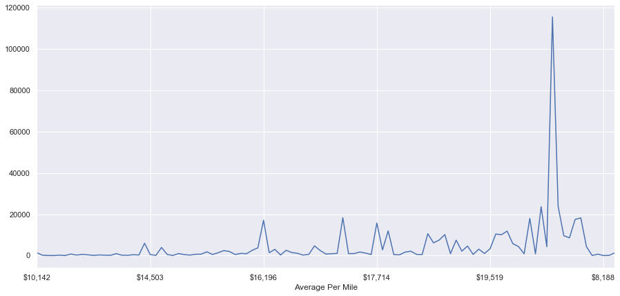
We see here that we both don’t have information for all of the cities in our crash data and that the most crashes are occuring in municipalities that fund their roads on average of 21,086. The real issue here is that the different values are so highly specific that they are just representing the different cities. We need to bin these values

result[['Currency']] = result[['Average Per Mile']].replace('[\$,]','',regex=True).astype(float)

result.head()

	Unnamed: 0	ACOUNT	ALCOHOL	BCOUNT	BICYCLE	CARTODB_ID	CCOUNT	CNTNAME	COMMERCIAL	COMMUNITY	...	YCORD	YEAR	YOUNG	County	Annual Amount	Road Miles	Average Per Mile	Unnamed: 5	Unnamed: 6	Currency
0	0	0	0	0	0	NaN	0	Washtenaw	NaN	Ann Arbor	...	42.28787	2017	0	Washtenaw	$7,535,530	296.70	$25,398	NaN	NaN	25398.0
1	1	0	0	0	0	NaN	0	Oakland	NaN	Brandon Twp	...	42.81026	2017	1	NaN	NaN	NaN	NaN	NaN	NaN	NaN
2	2	0	0	0	0	NaN	0	Oakland	NaN	Bloomfield Twp	...	42.61546	2017	1	NaN	NaN	NaN	NaN	NaN	NaN	NaN
3	3	0	0	0	0	NaN	0	Oakland	NaN	Orchard Lake Village	...	42.57882	2017	0	NaN	NaN	NaN	NaN	NaN	NaN	NaN
4	4	0	0	0	0	NaN	0	Livingston	NaN	Hartland Twp	...	42.65626	2017	0	NaN	NaN	NaN	NaN	NaN	NaN	NaN

5 rows × 68 columns

result['bin'] = pd.cut(result['Currency'], [0, 5000, 10000,15000,20000,25000,30000])

result.head()

	Unnamed: 0	ACOUNT	ALCOHOL	BCOUNT	BICYCLE	CARTODB_ID	CCOUNT	CNTNAME	COMMERCIAL	COMMUNITY	...	YEAR	YOUNG	County	Annual Amount	Road Miles	Average Per Mile	Unnamed: 5	Unnamed: 6	Currency	bin
0	0	0	0	0	0	NaN	0	Washtenaw	NaN	Ann Arbor	...	2017	0	Washtenaw	$7,535,530	296.70	$25,398	NaN	NaN	25398.0	(25000.0, 30000.0]
1	1	0	0	0	0	NaN	0	Oakland	NaN	Brandon Twp	...	2017	1	NaN	NaN	NaN	NaN	NaN	NaN	NaN	NaN
2	2	0	0	0	0	NaN	0	Oakland	NaN	Bloomfield Twp	...	2017	1	NaN	NaN	NaN	NaN	NaN	NaN	NaN	NaN
3	3	0	0	0	0	NaN	0	Oakland	NaN	Orchard Lake Village	...	2017	0	NaN	NaN	NaN	NaN	NaN	NaN	NaN	NaN
4	4	0	0	0	0	NaN	0	Livingston	NaN	Hartland Twp	...	2017	0	NaN	NaN	NaN	NaN	NaN	NaN	NaN	NaN

5 rows × 69 columns

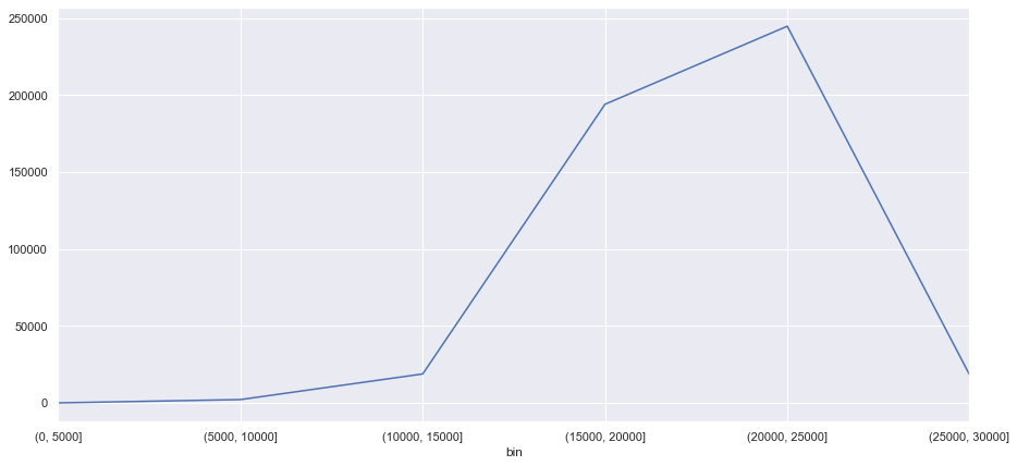
result.groupby('bin').size().sort_values(ascending =False)

bin
(20000, 25000]    244713
(15000, 20000]    194008
(10000, 15000]     18789
(25000, 30000]     18250
(5000, 10000]       2130
(0, 5000]              0
dtype: int64

fig, ax = plt.subplots(figsize=(15,7))
result.groupby('bin').size().plot(ax=ax)

<matplotlib.axes._subplots.AxesSubplot at 0x1199966a0>

Ann Arbor

Let’s look at a specific city in our data and see if the overarching trends are represented

df_aa = df.loc[df['COMMUNITY']=='Ann Arbor']

df_aa.head()

	Unnamed: 0	ACOUNT	ALCOHOL	BCOUNT	BICYCLE	CARTODB_ID	CCOUNT	CNTNAME	COMMERCIAL	COMMUNITY	...	UNITS	WEATHER	WEEKDAY	WORK_ZONE	X	XCORD	Y	YCORD	YEAR	YOUNG
0	0	0	0	0	0	NaN	0	Washtenaw	NaN	Ann Arbor	...	2	5	2	NaN	-83.771023	-83.77102	42.287878	42.28787	2017	0
21	21	0	0	0	0	NaN	0	Washtenaw	NaN	Ann Arbor	...	2	1	4	NaN	-83.707336	-83.70734	42.302537	42.30253	2017	0
52	52	0	0	1	0	NaN	1	Washtenaw	NaN	Ann Arbor	...	2	1	3	NaN	-83.749675	-83.74967	42.252243	42.25224	2017	0
121	121	0	0	1	0	NaN	0	Washtenaw	NaN	Ann Arbor	...	2	1	6	NaN	-83.739154	-83.73915	42.240915	42.24091	2017	1
131	131	0	0	0	0	NaN	0	Washtenaw	NaN	Ann Arbor	...	2	1	1	NaN	-83.735003	-83.73500	42.285408	42.28540	2017	0

5 rows × 61 columns

len(df_aa)

18250

709000 / 237

2991.5611814345993

2991.5611814345993 / 709000

0.0042194092827004225

.42 * 237

99.53999999999999

If all was equal, each city would have 2,991 crashes occur within their distinct city limits, but as mentioned above not all is equal.

237 * 2991

708867

We can see that 18,250 car cashes occurred within ann arbor city limits over the course of these five years in question.

18250 / 709000

0.025740479548660086

Each municipality should account for .4 percent of the crashes (if all was equal) but ann arbor is accounting for over 2.5 percent. This matches where ann arbor fell on our crash total list.

709000 * 0.025740479548660086

18250.0

aa_dates_result = df_aa.groupby('DATE_FULL').size().sort_values(ascending=False)

aa_dates_result

DATE_FULL
11/19/2014    48
01/01/2014    44
12/11/2017    43
03/07/2018    42
12/18/2014    39
01/27/2014    37
01/12/2018    37
03/13/2017    37
11/21/2015    36
04/17/2018    34
01/05/2015    33
02/24/2016    33
01/09/2014    32
01/28/2014    30
02/05/2014    29
02/09/2018    29
03/12/2014    28
01/29/2018    28
11/02/2017    28
01/09/2018    27
03/01/2016    26
01/16/2014    26
01/23/2014    26
11/21/2017    26
11/04/2016    25
01/29/2017    25
01/09/2015    25
11/18/2015    25
01/22/2014    25
10/31/2014    24
              ..
08/02/2015     2
07/26/2015     2
07/15/2018     2
07/13/2014     2
07/09/2016     2
07/04/2018     2
04/12/2014     2
07/03/2016     2
07/03/2015     2
02/17/2018     2
12/25/2016     1
04/07/2014     1
02/16/2015     1
03/16/2014     1
03/04/2018     1
01/02/2015     1
12/31/2016     1
08/28/2016     1
08/17/2014     1
11/27/2014     1
06/04/2017     1
11/26/2015     1
11/23/2017     1
11/22/2018     1
06/10/2018     1
06/21/2015     1
12/31/2017     1
07/04/2015     1
07/08/2018     1
05/24/2015     1
Length: 1823, dtype: int64

The day with the most crashes in ann arbor places third overall on the crash list for the entire region.

fig, ax = plt.subplots(figsize=(15,7))
aa_result_dates = df_aa.groupby('DATE_FULL').size().plot(ax=ax)

This figure follow the trends that appeared in the overall dates figure. We see spikes in car crashes on select days throughout the winter months.

fig, ax = plt.subplots(figsize=(15,7))
df_aa.groupby('HOUR').size().plot(ax=ax)

<matplotlib.axes._subplots.AxesSubplot at 0x11cfe5898>

The hourly distribution of crashes within the city follows the rush hour trend we identified in the total data

Ultimately, this sub sample of data seems to be representative of the full data.

High severity crashes

df.columns

Index(['Unnamed: 0', 'ACOUNT', 'ALCOHOL', 'BCOUNT', 'BICYCLE', 'CARTODB_ID',
       'CCOUNT', 'CNTNAME', 'COMMERCIAL', 'COMMUNITY', 'CRASHID', 'CRSHTYPEO',
       'DATE_FULL', 'DAY', 'DEER', 'DISTRACTED', 'DIS_CTRL_I', 'DRUG',
       'ELDERLY', 'EMERGENCY', 'FALINKID', 'FID', 'HIGH_SEVER', 'HITNRUN',
       'HOUR', 'HWY_CLSS_C', 'INTERROAD', 'INTR_INVL_', 'JURIS', 'KCOUNT',
       'LANEDEPART', 'LIGHTING', 'MAINROAD', 'MONTH', 'MOTORCYCLE', 'MP',
       'NFC', 'OBJECTID', 'OCCUPANTS', 'PEDESTRIAN', 'PR', 'PROPDAMG',
       'REDLIGHTRU', 'ROADCONDIT', 'ROADLANES', 'SCHOOLBUS', 'SEMMCD',
       'SPEEDLIMIT', 'SURFACE', 'TIME_FULL', 'TRAIN', 'UNITS', 'WEATHER',
       'WEEKDAY', 'WORK_ZONE', 'X', 'XCORD', 'Y', 'YCORD', 'YEAR', 'YOUNG'],
      dtype='object')

sev = df.loc[df['HIGH_SEVER']==1]

len(sev)

1782

Detroit vs Livonia

Conducting some evaluation of the genralizability of clustering groups

det = result.loc[result['COMMUNITY']=='Detroit']

liv = result.loc[result['COMMUNITY']=='Livonia']

det.head()

	Unnamed: 0	ACOUNT	ALCOHOL	BCOUNT	BICYCLE	CARTODB_ID	CCOUNT	CNTNAME	COMMERCIAL	COMMUNITY	...	YEAR	YOUNG	County	Annual Amount	Road Miles	Average Per Mile	Unnamed: 5	Unnamed: 6	Currency	bin
16	16	0	0	0	0	NaN	0	Wayne	NaN	Detroit	...	2017	0	Wayne	$54,202,186	2,570.50	$21,086	NaN	NaN	21086.0	(20000, 25000]
40	40	0	0	0	0	NaN	0	Wayne	NaN	Detroit	...	2017	1	Wayne	$54,202,186	2,570.50	$21,086	NaN	NaN	21086.0	(20000, 25000]
41	41	0	0	0	0	NaN	0	Wayne	NaN	Detroit	...	2017	0	Wayne	$54,202,186	2,570.50	$21,086	NaN	NaN	21086.0	(20000, 25000]
43	43	0	0	0	0	NaN	0	Wayne	NaN	Detroit	...	2017	0	Wayne	$54,202,186	2,570.50	$21,086	NaN	NaN	21086.0	(20000, 25000]
60	60	0	0	0	0	NaN	2	Wayne	NaN	Detroit	...	2017	0	Wayne	$54,202,186	2,570.50	$21,086	NaN	NaN	21086.0	(20000, 25000]

5 rows × 69 columns

len(det)

115539

len(liv)

18341

det.columns

Index(['Unnamed: 0', 'ACOUNT', 'ALCOHOL', 'BCOUNT', 'BICYCLE', 'CARTODB_ID',
       'CCOUNT', 'CNTNAME', 'COMMERCIAL', 'COMMUNITY', 'CRASHID', 'CRSHTYPEO',
       'DATE_FULL', 'DAY', 'DEER', 'DISTRACTED', 'DIS_CTRL_I', 'DRUG',
       'ELDERLY', 'EMERGENCY', 'FALINKID', 'FID', 'HIGH_SEVER', 'HITNRUN',
       'HOUR', 'HWY_CLSS_C', 'INTERROAD', 'INTR_INVL_', 'JURIS', 'KCOUNT',
       'LANEDEPART', 'LIGHTING', 'MAINROAD', 'MONTH', 'MOTORCYCLE', 'MP',
       'NFC', 'OBJECTID', 'OCCUPANTS', 'PEDESTRIAN', 'PR', 'PROPDAMG',
       'REDLIGHTRU', 'ROADCONDIT', 'ROADLANES', 'SCHOOLBUS', 'SEMMCD',
       'SPEEDLIMIT', 'SURFACE', 'TIME_FULL', 'TRAIN', 'UNITS', 'WEATHER',
       'WEEKDAY', 'WORK_ZONE', 'X', 'XCORD', 'Y', 'YCORD', 'YEAR', 'YOUNG',
       'County', 'Annual Amount', 'Road Miles', 'Average Per Mile',
       'Unnamed: 5', 'Unnamed: 6', 'Currency', 'bin'],
      dtype='object')

Let’s compare and contrast the rates at which key statistics occur.

det_bike = det.loc[det['BICYCLE']==1]
len(det_bike)

848

848 / 115539

0.007339513064852561

liv_bike = liv.loc[liv['BICYCLE']==1]
len(liv_bike)

117

117 / 18341

0.006379150537048144

det_bus = det.loc[det['SCHOOLBUS']==1]
len(det_bus)

320

320 / 115539

0.0027696275716424757

liv_bus = liv.loc[liv['SCHOOLBUS']==1]
len(liv_bus)

79

79 / 18341

0.004307289678861567

det_moto = det.loc[det['MOTORCYCLE']==1]
len(det_moto)

1068

1068 / 115539

0.009243632020356763

liv_moto = liv.loc[liv['MOTORCYCLE']==1]
len(liv_moto)

126

126 / 18341

0.006869854424513385

det_old = det.loc[det['ELDERLY']==1]

len(det_old)

13205

13205 / 115539

0.11429041276105904

liv_old = liv.loc[liv['ELDERLY']==1]

len(liv_old)

3671

3671 / 18341

0.20015266343165586

det_young = det.loc[det['YOUNG']==1]

len(det_young)

29981

29981 / 115539

0.25948813820441585

liv_young = liv.loc[liv['YOUNG']==1]

len(liv_young)

6301

6301 / 18341

0.34354724387983204

det_alc = det.loc[det['ALCOHOL']==1]

len(det_alc)

2323

2323 / 115539

0.020105765152892096

liv_alc = liv.loc[liv['ALCOHOL']==1]

len(liv_alc)

470

470 / 18341

0.025625647456518182

det_drug = det.loc[det['DRUG']==1]

len(det_drug)

626

626 / 115539

0.005418083937025593

liv_drug = liv.loc[liv['DRUG']==1]

len(liv_drug)

149

149 / 18341

0.008123875470257893

det_sev = det.loc[det['CRSHTYPEO']==1]

len(det_sev)

16170

16170 / 115539

0.13995274322955886

liv_sev = liv.loc[liv['CRSHTYPEO']==1]

len(liv_sev)

1782

1782 / 18341

0.09715936971811788

det_dis = det.loc[det['DISTRACTED']==1]

len(det_dis)

3678

3678 / 115539

0.031833406901565706

liv_dis = liv.loc[liv['DISTRACTED']==1]

len(liv_dis)

577

577 / 18341

0.03145957145193828

det['bin']

16        (20000, 25000]
40        (20000, 25000]
41        (20000, 25000]
43        (20000, 25000]
60        (20000, 25000]
68        (20000, 25000]
76        (20000, 25000]
94        (20000, 25000]
108       (20000, 25000]
109       (20000, 25000]
128       (20000, 25000]
156       (20000, 25000]
175       (20000, 25000]
179       (20000, 25000]
180       (20000, 25000]
182       (20000, 25000]
190       (20000, 25000]
192       (20000, 25000]
198       (20000, 25000]
209       (20000, 25000]
214       (20000, 25000]
218       (20000, 25000]
224       (20000, 25000]
235       (20000, 25000]
245       (20000, 25000]
247       (20000, 25000]
250       (20000, 25000]
251       (20000, 25000]
254       (20000, 25000]
258       (20000, 25000]
               ...      
709804    (20000, 25000]
709817    (20000, 25000]
709818    (20000, 25000]
709824    (20000, 25000]
709825    (20000, 25000]
709827    (20000, 25000]
709828    (20000, 25000]
709830    (20000, 25000]
709831    (20000, 25000]
709833    (20000, 25000]
709834    (20000, 25000]
709840    (20000, 25000]
709842    (20000, 25000]
709851    (20000, 25000]
709852    (20000, 25000]
709855    (20000, 25000]
709857    (20000, 25000]
709858    (20000, 25000]
709863    (20000, 25000]
709865    (20000, 25000]
709866    (20000, 25000]
709870    (20000, 25000]
709875    (20000, 25000]
709878    (20000, 25000]
709879    (20000, 25000]
709884    (20000, 25000]
709889    (20000, 25000]
709895    (20000, 25000]
709897    (20000, 25000]
709898    (20000, 25000]
Name: bin, Length: 115539, dtype: category
Categories (6, interval[int64]): [(0, 5000] < (5000, 10000] < (10000, 15000] < (15000, 20000] < (20000, 25000] < (25000, 30000]]

liv['bin']

15        (15000, 20000]
27        (15000, 20000]
72        (15000, 20000]
98        (15000, 20000]
107       (15000, 20000]
133       (15000, 20000]
162       (15000, 20000]
178       (15000, 20000]
197       (15000, 20000]
213       (15000, 20000]
276       (15000, 20000]
285       (15000, 20000]
309       (15000, 20000]
340       (15000, 20000]
357       (15000, 20000]
371       (15000, 20000]
396       (15000, 20000]
429       (15000, 20000]
450       (15000, 20000]
451       (15000, 20000]
461       (15000, 20000]
464       (15000, 20000]
470       (15000, 20000]
476       (15000, 20000]
485       (15000, 20000]
487       (15000, 20000]
489       (15000, 20000]
495       (15000, 20000]
508       (15000, 20000]
510       (15000, 20000]
               ...      
708660    (15000, 20000]
708677    (15000, 20000]
708718    (15000, 20000]
708720    (15000, 20000]
708787    (15000, 20000]
708864    (15000, 20000]
708902    (15000, 20000]
708924    (15000, 20000]
709028    (15000, 20000]
709042    (15000, 20000]
709079    (15000, 20000]
709081    (15000, 20000]
709092    (15000, 20000]
709093    (15000, 20000]
709149    (15000, 20000]
709162    (15000, 20000]
709220    (15000, 20000]
709269    (15000, 20000]
709323    (15000, 20000]
709337    (15000, 20000]
709427    (15000, 20000]
709441    (15000, 20000]
709443    (15000, 20000]
709590    (15000, 20000]
709618    (15000, 20000]
709794    (15000, 20000]
709822    (15000, 20000]
709850    (15000, 20000]
709853    (15000, 20000]
709881    (15000, 20000]
Name: bin, Length: 18341, dtype: category
Categories (6, interval[int64]): [(0, 5000] < (5000, 10000] < (10000, 15000] < (15000, 20000] < (20000, 25000] < (25000, 30000]]