
Project 01: Exploratory Data Analysis
Zillow Housing Prices Exploratory Data Analysis
Load Data
import pandas as pd
import numpy as np
import seaborn as sns
state_data = pd.read_csv("zecon/State_time_series.csv",parse_dates=True)
print(len(state_data.columns))
print(len(state_data))
82
13212
state_data = state_data[['Date','RegionName','ZHVI_1bedroom','ZHVI_2bedroom','ZHVI_3bedroom','ZHVI_4bedroom','ZHVI_BottomTier','ZHVI_CondoCoop','ZHVI_MiddleTier','ZHVI_SingleFamilyResidence','ZHVI_TopTier']]
state_data["Date"] = pd.to_datetime(state_data["Date"])
state_data['Year'] = state_data['Date'].dt.year
state_data['Month'] = state_data['Date'].dt.month
cross_data = pd.read_csv("zecon/cities_crosswalk.csv")
#cross_data.head()
cities_data = pd.read_csv("zecon/City_time_series.csv")
cities_data.head()
| Date | RegionName | InventorySeasonallyAdjusted_AllHomes | InventoryRaw_AllHomes | MedianListingPricePerSqft_1Bedroom | MedianListingPricePerSqft_2Bedroom | MedianListingPricePerSqft_3Bedroom | MedianListingPricePerSqft_4Bedroom | MedianListingPricePerSqft_5BedroomOrMore | MedianListingPricePerSqft_AllHomes | ... | ZHVI_BottomTier | ZHVI_CondoCoop | ZHVI_MiddleTier | ZHVI_SingleFamilyResidence | ZHVI_TopTier | ZRI_AllHomes | ZRI_AllHomesPlusMultifamily | ZriPerSqft_AllHomes | Zri_MultiFamilyResidenceRental | Zri_SingleFamilyResidenceRental | |
|---|---|---|---|---|---|---|---|---|---|---|---|---|---|---|---|---|---|---|---|---|---|
| 0 | 1996-04-30 | abbottstownadamspa | NaN | NaN | NaN | NaN | NaN | NaN | NaN | NaN | ... | NaN | NaN | NaN | NaN | 108700.0 | NaN | NaN | NaN | NaN | NaN |
| 1 | 1996-04-30 | aberdeenbinghamid | NaN | NaN | NaN | NaN | NaN | NaN | NaN | NaN | ... | NaN | NaN | NaN | NaN | 168400.0 | NaN | NaN | NaN | NaN | NaN |
| 2 | 1996-04-30 | aberdeenharfordmd | NaN | NaN | NaN | NaN | NaN | NaN | NaN | NaN | ... | 81300.0 | 137900.0 | 109600.0 | 108600.0 | 147900.0 | NaN | NaN | NaN | NaN | NaN |
| 3 | 1996-04-30 | aberdeenmonroems | NaN | NaN | NaN | NaN | NaN | NaN | NaN | NaN | ... | NaN | NaN | NaN | NaN | 74500.0 | NaN | NaN | NaN | NaN | NaN |
| 4 | 1996-04-30 | aberdeenmoorenc | NaN | NaN | NaN | NaN | NaN | NaN | NaN | NaN | ... | NaN | NaN | NaN | NaN | 131100.0 | NaN | NaN | NaN | NaN | NaN |
5 rows × 81 columns
print(len(cities_data.columns))
print(len(cities_data))
81
3762566
cities_data["Date"] = pd.to_datetime(cities_data["Date"])
cities_data['Year'] = cities_data['Date'].dt.year
cities_data['Month'] = cities_data['Date'].dt.month
city_state_data = cities_data.join(cross_data.set_index('Unique_City_ID'), on='RegionName')
Michigan
data_michigan = state_data.loc[state_data['RegionName'] == 'Michigan']
year_plot = sns.barplot(x="Year", y="ZHVI_MiddleTier", data=data_michigan)
year_plot.set_xticklabels(year_plot.get_xticklabels(), rotation=90)
[Text(0, 0, '1996'),
 Text(0, 0, '1997'),
 Text(0, 0, '1998'),
 Text(0, 0, '1999'),
 Text(0, 0, '2000'),
 Text(0, 0, '2001'),
 Text(0, 0, '2002'),
 Text(0, 0, '2003'),
 Text(0, 0, '2004'),
 Text(0, 0, '2005'),
 Text(0, 0, '2006'),
 Text(0, 0, '2007'),
 Text(0, 0, '2008'),
 Text(0, 0, '2009'),
 Text(0, 0, '2010'),
 Text(0, 0, '2011'),
 Text(0, 0, '2012'),
 Text(0, 0, '2013'),
 Text(0, 0, '2014'),
 Text(0, 0, '2015'),
 Text(0, 0, '2016'),
 Text(0, 0, '2017')]

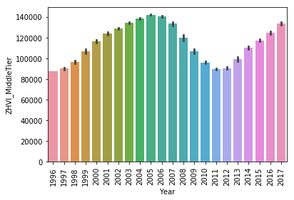
This graph shows the median housing price within michigan over the course of the dataset. It accurately shows the 2008 recession and therefore is fairly reasonable to believe.
Examining the Country in 2017
country_df = state_data[["RegionName","ZHVI_MiddleTier","Year"]]
country_df = country_df.loc[country_df["Year"]==2017]
country_df = country_df.dropna()
#country_df
state_plot = sns.barplot(x="RegionName", y="ZHVI_MiddleTier", data=country_df)
state_plot.set_xticklabels(state_plot.get_xticklabels(), rotation=90,size=7)
[Text(0, 0, 'Alabama'),
 Text(0, 0, 'Alaska'),
 Text(0, 0, 'Arizona'),
 Text(0, 0, 'Arkansas'),
 Text(0, 0, 'California'),
 Text(0, 0, 'Colorado'),
 Text(0, 0, 'Connecticut'),
 Text(0, 0, 'Delaware'),
 Text(0, 0, 'DistrictofColumbia'),
 Text(0, 0, 'Florida'),
 Text(0, 0, 'Georgia'),
 Text(0, 0, 'Hawaii'),
 Text(0, 0, 'Idaho'),
 Text(0, 0, 'Illinois'),
 Text(0, 0, 'Indiana'),
 Text(0, 0, 'Iowa'),
 Text(0, 0, 'Kansas'),
 Text(0, 0, 'Kentucky'),
 Text(0, 0, 'Maine'),
 Text(0, 0, 'Maryland'),
 Text(0, 0, 'Massachusetts'),
 Text(0, 0, 'Michigan'),
 Text(0, 0, 'Minnesota'),
 Text(0, 0, 'Mississippi'),
 Text(0, 0, 'Missouri'),
 Text(0, 0, 'Montana'),
 Text(0, 0, 'Nebraska'),
 Text(0, 0, 'Nevada'),
 Text(0, 0, 'NewHampshire'),
 Text(0, 0, 'NewJersey'),
 Text(0, 0, 'NewMexico'),
 Text(0, 0, 'NewYork'),
 Text(0, 0, 'NorthCarolina'),
 Text(0, 0, 'NorthDakota'),
 Text(0, 0, 'Ohio'),
 Text(0, 0, 'Oklahoma'),
 Text(0, 0, 'Oregon'),
 Text(0, 0, 'Pennsylvania'),
 Text(0, 0, 'RhodeIsland'),
 Text(0, 0, 'SouthCarolina'),
 Text(0, 0, 'SouthDakota'),
 Text(0, 0, 'Tennessee'),
 Text(0, 0, 'Texas'),
 Text(0, 0, 'Utah'),
 Text(0, 0, 'Vermont'),
 Text(0, 0, 'Virginia'),
 Text(0, 0, 'Washington'),
 Text(0, 0, 'WestVirginia'),
 Text(0, 0, 'Wisconsin'),
 Text(0, 0, 'Wyoming')]

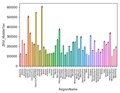
This graph makes intuitive sense as the states as the top are Hawaii and California along with Washington D.C. The cheapes states are West Virginia, Mississippi, and Oklahoma.
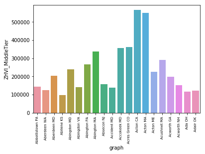
QUESTION ONE: I’d like to find out where is the most expensive city to live in 2017 and where is the least expensive.
Take the values for the state data set prices and determine which are the max and min prices overall. I can then visualize these through creating a scatter plot in plot.ly or with d3 that maps the max and min for each state’s prices to show the spread and differences for each of the states
max_min_cities = city_state_data
q1_a = max_min_cities[["Date","RegionName","ZHVIPerSqft_AllHomes","ZHVI_BottomTier","ZHVI_MiddleTier","ZHVI_SingleFamilyResidence","ZHVI_TopTier","Month","Year","City","County","State"]]
q1_a = q1_a.dropna()
#specific data for question
q1_a = q1_a.loc[q1_a['Year'] == 2017]
q1_a = q1_a.loc[q1_a['Month']== 5]
q1_a.head()
| Date | RegionName | ZHVIPerSqft_AllHomes | ZHVI_BottomTier | ZHVI_MiddleTier | ZHVI_SingleFamilyResidence | ZHVI_TopTier | Month | Year | City | County | State | |
|---|---|---|---|---|---|---|---|---|---|---|---|---|
| 3630515 | 2017-05-31 | abbottstownadamspa | 121.0 | 133100.0 | 143800.0 | 143800.0 | 166700.0 | 5 | 2017 | Abbottstown | Adams | PA |
| 3630518 | 2017-05-31 | aberdeengrays_harborwa | 82.0 | 79100.0 | 123700.0 | 123800.0 | 199200.0 | 5 | 2017 | Aberdeen | Grays Harbor | WA |
| 3630519 | 2017-05-31 | aberdeenharfordmd | 142.0 | 144300.0 | 204100.0 | 202500.0 | 298300.0 | 5 | 2017 | Aberdeen | Harford | MD |
| 3630523 | 2017-05-31 | abilenedickinsonks | 72.0 | 65000.0 | 96700.0 | 96700.0 | 146100.0 | 5 | 2017 | Abilene | Dickinson | KS |
| 3630525 | 2017-05-31 | abingdonharfordmd | 151.0 | 184400.0 | 238600.0 | 241200.0 | 317000.0 | 5 | 2017 | Abingdon | Harford | MD |
q1_a['graph'] = q1_a["City"] + " " + q1_a["State"]
q1_a.head()
| Date | RegionName | ZHVIPerSqft_AllHomes | ZHVI_BottomTier | ZHVI_MiddleTier | ZHVI_SingleFamilyResidence | ZHVI_TopTier | Month | Year | City | County | State | graph | |
|---|---|---|---|---|---|---|---|---|---|---|---|---|---|
| 3630515 | 2017-05-31 | abbottstownadamspa | 121.0 | 133100.0 | 143800.0 | 143800.0 | 166700.0 | 5 | 2017 | Abbottstown | Adams | PA | Abbottstown PA |
| 3630518 | 2017-05-31 | aberdeengrays_harborwa | 82.0 | 79100.0 | 123700.0 | 123800.0 | 199200.0 | 5 | 2017 | Aberdeen | Grays Harbor | WA | Aberdeen WA |
| 3630519 | 2017-05-31 | aberdeenharfordmd | 142.0 | 144300.0 | 204100.0 | 202500.0 | 298300.0 | 5 | 2017 | Aberdeen | Harford | MD | Aberdeen MD |
| 3630523 | 2017-05-31 | abilenedickinsonks | 72.0 | 65000.0 | 96700.0 | 96700.0 | 146100.0 | 5 | 2017 | Abilene | Dickinson | KS | Abilene KS |
| 3630525 | 2017-05-31 | abingdonharfordmd | 151.0 | 184400.0 | 238600.0 | 241200.0 | 317000.0 | 5 | 2017 | Abingdon | Harford | MD | Abingdon MD |
#q1_a_vis = q1_a.sort_values("ton",ascending=False).head(5)
q1_a_vis = q1_a[["ZHVI_MiddleTier","City","County","State","graph"]]
q1_a_vis.sort_values("ZHVI_MiddleTier",ascending=False)
| ZHVI_MiddleTier | City | County | State | graph | |
|---|---|---|---|---|---|
| 3631033 | 6399100.0 | Atherton | San Mateo | CA | Atherton CA |
| 3638742 | 4421300.0 | Los Altos Hills | Santa Clara | CA | Los Altos Hills CA |
| 3636938 | 4243800.0 | Hillsborough | San Mateo | CA | Hillsborough CA |
| 3646055 | 4099600.0 | Water Mill | Suffolk | NY | Water Mill NY |
| 3642104 | 3797800.0 | Portola Valley | San Mateo | CA | Portola Valley CA |
| 3631519 | 3562400.0 | Belvedere | Marin | CA | Belvedere CA |
| 3646916 | 3395200.0 | Woodside | San Mateo | CA | Woodside CA |
| 3636873 | 3183000.0 | Hidden Hills | Los Angeles | CA | Hidden Hills CA |
| 3631662 | 3042500.0 | Beverly Hills | Los Angeles | CA | Beverly Hills CA |
| 3644200 | 3020100.0 | Stanford | Santa Clara | CA | Stanford CA |
| 3639005 | 2892100.0 | Malibu | Los Angeles | CA | Malibu CA |
| 3638743 | 2891400.0 | Los Altos | Santa Clara | CA | Los Altos CA |
| 3639885 | 2881600.0 | Monte Sereno | Santa Clara | CA | Monte Sereno CA |
| 3641384 | 2645700.0 | Palo Alto | Santa Clara | CA | Palo Alto CA |
| 3642330 | 2594900.0 | Rancho Santa Fe | San Diego | CA | Rancho Santa Fe CA |
| 3647004 | 2558600.0 | Yarrow Point | King | WA | Yarrow Point WA |
| 3639434 | 2541700.0 | Medina | King | WA | Medina WA |
| 3643292 | 2518200.0 | Saratoga | Santa Clara | CA | Saratoga CA |
| 3644754 | 2507100.0 | Tiburon | Marin | CA | Tiburon CA |
| 3633293 | 2428000.0 | Clyde Hill | King | WA | Clyde Hill WA |
| 3643225 | 2285300.0 | Sands Point | Nassau | NY | Sands Point NY |
| 3643202 | 2244100.0 | San Marino | Los Angeles | CA | San Marino CA |
| 3639048 | 2242500.0 | Manhattan Beach | Los Angeles | CA | Manhattan Beach CA |
| 3641066 | 2225600.0 | Old Westbury | Nassau | NY | Old Westbury NY |
| 3641733 | 2145900.0 | Piedmont | Alameda | CA | Piedmont CA |
| 3634079 | 2107900.0 | Del Mar | San Diego | CA | Del Mar CA |
| 3632968 | 2055600.0 | Cherry Hills Village | Arapahoe | CO | Cherry Hills Village CO |
| 3637730 | 2053800.0 | Kentfield | Marin | CA | Kentfield CA |
| 3641886 | 2020800.0 | Plandome | Nassau | NY | Plandome NY |
| 3641391 | 2011400.0 | Palos Verdes Estates | Los Angeles | CA | Palos Verdes Estates CA |
| ... | ... | ... | ... | ... | ... |
| 3639045 | 48700.0 | Mangum | Greer | OK | Mangum OK |
| 3639365 | 48600.0 | McDonald Chapel | Jefferson | AL | McDonald Chapel AL |
| 3634409 | 48300.0 | Duquesne | Allegheny | PA | Duquesne PA |
| 3639349 | 47800.0 | McAdoo | Schuylkill | PA | McAdoo PA |
| 3635506 | 47700.0 | Frackville | Schuylkill | PA | Frackville PA |
| 3638956 | 47400.0 | Madison | Madison | IL | Madison IL |
| 3638559 | 47400.0 | Lipscomb | Jefferson | AL | Lipscomb AL |
| 3635101 | 47100.0 | Fairmont City | Saint Clair | IL | Fairmont City IL |
| 3640833 | 46800.0 | Northridge | Montgomery | OH | Northridge OH |
| 3634676 | 46400.0 | Edgewater | Jefferson | AL | Edgewater AL |
| 3645715 | 46400.0 | Venice | Madison | IL | Venice IL |
| 3642349 | 45700.0 | Rankin | Allegheny | PA | Rankin PA |
| 3640478 | 45600.0 | New Philadelphia | Schuylkill | PA | New Philadelphia PA |
| 3645984 | 45500.0 | Warren | Trumbull | OH | Warren OH |
| 3635049 | 44400.0 | Experiment | Spalding | GA | Experiment GA |
| 3632854 | 44300.0 | Centreville | Saint Clair | IL | Centreville IL |
| 3635433 | 44000.0 | Fort McKinley | Montgomery | OH | Fort McKinley OH |
| 3639752 | 43300.0 | Minersville | Schuylkill | PA | Minersville PA |
| 3634580 | 42800.0 | East Saint Louis | Saint Clair | IL | East Saint Louis IL |
| 3632527 | 42300.0 | Campbell | Mahoning | OH | Campbell OH |
| 3644592 | 41900.0 | Tamaqua | Schuylkill | PA | Tamaqua PA |
| 3634178 | 41400.0 | Detroit | Wayne | MI | Detroit MI |
| 3643602 | 39800.0 | Shenandoah Heights | Schuylkill | PA | Shenandoah Heights PA |
| 3633307 | 38300.0 | Coaldale | Schuylkill | PA | Coaldale PA |
| 3643039 | 37600.0 | Saint Clair | Schuylkill | PA | Saint Clair PA |
| 3637573 | 37600.0 | Johnstown | Cambria | PA | Johnstown PA |
| 3635895 | 32900.0 | Girardville | Schuylkill | PA | Girardville PA |
| 3630999 | 31600.0 | Ashland | Schuylkill | PA | Ashland PA |
| 3643607 | 31100.0 | Shenandoah | Schuylkill | PA | Shenandoah PA |
| 3638981 | 30100.0 | Mahanoy City | Schuylkill | PA | Mahanoy City PA |
9886 rows × 5 columns
q1_a_vis = q1_a_vis.head(20)
q1_a_plot = sns.barplot(x="graph", y="ZHVI_MiddleTier", data=q1_a_vis)
q1_a_plot.set_xticklabels(q1_a_plot.get_xticklabels(), rotation=90,size=7)
[Text(0, 0, 'Abbottstown PA'),
 Text(0, 0, 'Aberdeen WA'),
 Text(0, 0, 'Aberdeen MD'),
 Text(0, 0, 'Abilene KS'),
 Text(0, 0, 'Abingdon MD'),
 Text(0, 0, 'Abingdon VA'),
 Text(0, 0, 'Abington PA'),
 Text(0, 0, 'Abington MA'),
 Text(0, 0, 'Absecon NJ'),
 Text(0, 0, 'Accident MD'),
 Text(0, 0, 'Accokeek MD'),
 Text(0, 0, 'Acres Green CO'),
 Text(0, 0, 'Acton CA'),
 Text(0, 0, 'Acton MA'),
 Text(0, 0, 'Acton ME'),
 Text(0, 0, 'Acushnet MA'),
 Text(0, 0, 'Acworth GA'),
 Text(0, 0, 'Acworth NH'),
 Text(0, 0, 'Ada OH'),
 Text(0, 0, 'Adair OK')]

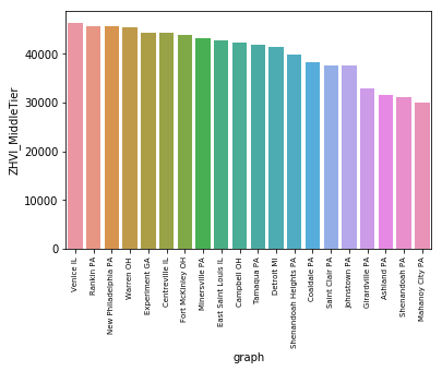
q1_b_vis = q1_a.sort_values("ZHVI_MiddleTier",ascending=False).tail(20)
q1_b_vis[["ZHVI_MiddleTier","City","County","State"]]
| ZHVI_MiddleTier | City | County | State | |
|---|---|---|---|---|
| 3645715 | 46400.0 | Venice | Madison | IL |
| 3642349 | 45700.0 | Rankin | Allegheny | PA |
| 3640478 | 45600.0 | New Philadelphia | Schuylkill | PA |
| 3645984 | 45500.0 | Warren | Trumbull | OH |
| 3635049 | 44400.0 | Experiment | Spalding | GA |
| 3632854 | 44300.0 | Centreville | Saint Clair | IL |
| 3635433 | 44000.0 | Fort McKinley | Montgomery | OH |
| 3639752 | 43300.0 | Minersville | Schuylkill | PA |
| 3634580 | 42800.0 | East Saint Louis | Saint Clair | IL |
| 3632527 | 42300.0 | Campbell | Mahoning | OH |
| 3644592 | 41900.0 | Tamaqua | Schuylkill | PA |
| 3634178 | 41400.0 | Detroit | Wayne | MI |
| 3643602 | 39800.0 | Shenandoah Heights | Schuylkill | PA |
| 3633307 | 38300.0 | Coaldale | Schuylkill | PA |
| 3643039 | 37600.0 | Saint Clair | Schuylkill | PA |
| 3637573 | 37600.0 | Johnstown | Cambria | PA |
| 3635895 | 32900.0 | Girardville | Schuylkill | PA |
| 3630999 | 31600.0 | Ashland | Schuylkill | PA |
| 3643607 | 31100.0 | Shenandoah | Schuylkill | PA |
| 3638981 | 30100.0 | Mahanoy City | Schuylkill | PA |
q1_b_plot = sns.barplot(x="graph", y="ZHVI_MiddleTier", data=q1_b_vis)
q1_b_plot.set_xticklabels(q1_b_plot.get_xticklabels(), rotation=90,size=7)
[Text(0, 0, 'Venice IL'),
 Text(0, 0, 'Rankin PA'),
 Text(0, 0, 'New Philadelphia PA'),
 Text(0, 0, 'Warren OH'),
 Text(0, 0, 'Experiment GA'),
 Text(0, 0, 'Centreville IL'),
 Text(0, 0, 'Fort McKinley OH'),
 Text(0, 0, 'Minersville PA'),
 Text(0, 0, 'East Saint Louis IL'),
 Text(0, 0, 'Campbell OH'),
 Text(0, 0, 'Tamaqua PA'),
 Text(0, 0, 'Detroit MI'),
 Text(0, 0, 'Shenandoah Heights PA'),
 Text(0, 0, 'Coaldale PA'),
 Text(0, 0, 'Saint Clair PA'),
 Text(0, 0, 'Johnstown PA'),
 Text(0, 0, 'Girardville PA'),
 Text(0, 0, 'Ashland PA'),
 Text(0, 0, 'Shenandoah PA'),
 Text(0, 0, 'Mahanoy City PA')]

QUESTION 2: Explore each states’ cities and figure out where the most expensive and least expensive places to live are for 2017 in each state.
Take the values for the city data set and determine which city has the highest price per square foot in each state. Then create scatterplot with matplotlib to measure each states’ individual cities and show which are the most expensive and least expensive parts of the state.
q2_a = city_state_data.loc[city_state_data['Year'] == 2017]
q2_a = q2_a.loc[q2_a['Month'] == 5]
q2_a = q2_a[["Date","ZHVIPerSqft_AllHomes","Month","Year","City","County","State"]]
q2_a = q2_a.dropna()
q2_a.head()
| Date | ZHVIPerSqft_AllHomes | Month | Year | City | County | State | |
|---|---|---|---|---|---|---|---|
| 3630513 | 2017-05-31 | 92.0 | 5 | 2017 | Abbeville | Lafayette | MS |
| 3630515 | 2017-05-31 | 121.0 | 5 | 2017 | Abbottstown | Adams | PA |
| 3630516 | 2017-05-31 | 90.0 | 5 | 2017 | Aberdeen | Bingham | ID |
| 3630518 | 2017-05-31 | 82.0 | 5 | 2017 | Aberdeen | Grays Harbor | WA |
| 3630519 | 2017-05-31 | 142.0 | 5 | 2017 | Aberdeen | Harford | MD |
q2_max = q2_a.groupby(q2_a["State"],sort=False)["ZHVIPerSqft_AllHomes"].transform(max) == q2_a["ZHVIPerSqft_AllHomes"]
q2_a[q2_max]
| Date | ZHVIPerSqft_AllHomes | Month | Year | City | County | State | |
|---|---|---|---|---|---|---|---|
| 3630933 | 2017-05-31 | 463.0 | 5 | 2017 | Arlington | Arlington | VA |
| 3631011 | 2017-05-31 | 1132.0 | 5 | 2017 | Aspen | Pitkin | CO |
| 3631033 | 2017-05-31 | 1746.0 | 5 | 2017 | Atherton | San Mateo | CA |
| 3631451 | 2017-05-31 | 363.0 | 5 | 2017 | Belle Meade | Davidson | TN |
| 3631463 | 2017-05-31 | 172.0 | 5 | 2017 | Bellefonte | New Castle | DE |
| 3631707 | 2017-05-31 | 251.0 | 5 | 2017 | Birmingham | Oakland | MI |
| 3632352 | 2017-05-31 | 200.0 | 5 | 2017 | Burlington | Chittenden | VT |
| 3632520 | 2017-05-31 | 147.0 | 5 | 2017 | Cammack Village | Pulaski | AR |
| 3632944 | 2017-05-31 | 137.0 | 5 | 2017 | Cheat Lake | Monongalia | WV |
| 3633019 | 2017-05-31 | 647.0 | 5 | 2017 | Chevy Chase Village | Montgomery | MD |
| 3633408 | 2017-05-31 | 192.0 | 5 | 2017 | Colonial Pine Hills | Pennington | SD |
| 3634333 | 2017-05-31 | 279.0 | 5 | 2017 | Druid Hills | Dekalb | GA |
| 3635022 | 2017-05-31 | 166.0 | 5 | 2017 | Evansville | Natrona | WY |
| 3635274 | 2017-05-31 | 1098.0 | 5 | 2017 | Fisher Island | Miami-Dade | FL |
| 3635520 | 2017-05-31 | 264.0 | 5 | 2017 | Frankfort | Franklin | KY |
| 3635710 | 2017-05-31 | 210.0 | 5 | 2017 | Gallatin Gateway | Gallatin | MT |
| 3635938 | 2017-05-31 | 426.0 | 5 | 2017 | Glenbrook | Douglas | NV |
| 3636293 | 2017-05-31 | 579.0 | 5 | 2017 | Greenwich | Fairfield | CT |
| 3636423 | 2017-05-31 | 704.0 | 5 | 2017 | Haleiwa | Honolulu | HI |
| 3637616 | 2017-05-31 | 210.0 | 5 | 2017 | Juneau | Juneau | AK |
| 3637706 | 2017-05-31 | 417.0 | 5 | 2017 | Kenilworth | Cook | IL |
| 3637754 | 2017-05-31 | 388.0 | 5 | 2017 | Ketchum | Blaine | ID |
| 3637984 | 2017-05-31 | 265.0 | 5 | 2017 | Ladue | Saint Louis | MO |
| 3638509 | 2017-05-31 | 215.0 | 5 | 2017 | Lincoln | Burleigh | ND |
| 3638957 | 2017-05-31 | 110.0 | 5 | 2017 | Madison | Madison | MS |
| 3639099 | 2017-05-31 | 207.0 | 5 | 2017 | Maple Bluff | Dane | WI |
| 3639434 | 2017-05-31 | 764.0 | 5 | 2017 | Medina | King | WA |
| 3639508 | 2017-05-31 | 175.0 | 5 | 2017 | Meridian Hills | Marion | IN |
| 3639784 | 2017-05-31 | 244.0 | 5 | 2017 | Mission Hills | Johnson | KS |
| 3640113 | 2017-05-31 | 295.0 | 5 | 2017 | Mount Olympus | Salt Lake | UT |
| 3640405 | 2017-05-31 | 426.0 | 5 | 2017 | New Castle | Rockingham | NH |
| 3640473 | 2017-05-31 | 156.0 | 5 | 2017 | New Orleans | Orleans | LA |
| 3640498 | 2017-05-31 | 590.0 | 5 | 2017 | New Shoreham | Washington | RI |
| 3640604 | 2017-05-31 | 171.0 | 5 | 2017 | Nichols Hills | Oklahoma | OK |
| 3641023 | 2017-05-31 | 330.0 | 5 | 2017 | Ogunquit | York | ME |
| 3641134 | 2017-05-31 | 265.0 | 5 | 2017 | Orange Beach | Baldwin | AL |
| 3641419 | 2017-05-31 | 377.0 | 5 | 2017 | Paradise Valley | Maricopa | AZ |
| 3642101 | 2017-05-31 | 330.0 | 5 | 2017 | Portland | Multnomah | OR |
| 3642301 | 2017-05-31 | 256.0 | 5 | 2017 | Radnor | Delaware | PA |
| 3642803 | 2017-05-31 | 414.0 | 5 | 2017 | Rollingwood | Travis | TX |
| 3643266 | 2017-05-31 | 195.0 | 5 | 2017 | Santa Fe | Santa Fe | NM |
| 3644306 | 2017-05-31 | 763.0 | 5 | 2017 | Stone Harbor | Cape May | NJ |
| 3644416 | 2017-05-31 | 606.0 | 5 | 2017 | Sullivans Island | Charleston | SC |
| 3644695 | 2017-05-31 | 262.0 | 5 | 2017 | The Village of Indian Hill | Hamilton | OH |
| 3644830 | 2017-05-31 | 353.0 | 5 | 2017 | Tonka Bay | Hennepin | MN |
| 3645147 | 2017-05-31 | 781.0 | 5 | 2017 | Town of Nantucket | Nantucket | MA |
| 3645562 | 2017-05-31 | 187.0 | 5 | 2017 | University Heights | Johnson | IA |
| 3646033 | 2017-05-31 | 493.0 | 5 | 2017 | Washington | District of Columbia | DC |
| 3646055 | 2017-05-31 | 1185.0 | 5 | 2017 | Water Mill | Suffolk | NY |
| 3646070 | 2017-05-31 | 158.0 | 5 | 2017 | Waterloo | Douglas | NE |
| 3646964 | 2017-05-31 | 555.0 | 5 | 2017 | Wrightsville Beach | New Hanover | NC |
max_graph = sns.barplot(x="State", y="ZHVIPerSqft_AllHomes", data=q2_a[q2_max])
max_graph.set_xticklabels(max_graph.get_xticklabels(), rotation=90,size=7)
[Text(0, 0, 'VA'),
 Text(0, 0, 'CO'),
 Text(0, 0, 'CA'),
 Text(0, 0, 'TN'),
 Text(0, 0, 'DE'),
 Text(0, 0, 'MI'),
 Text(0, 0, 'VT'),
 Text(0, 0, 'AR'),
 Text(0, 0, 'WV'),
 Text(0, 0, 'MD'),
 Text(0, 0, 'SD'),
 Text(0, 0, 'GA'),
 Text(0, 0, 'WY'),
 Text(0, 0, 'FL'),
 Text(0, 0, 'KY'),
 Text(0, 0, 'MT'),
 Text(0, 0, 'NV'),
 Text(0, 0, 'CT'),
 Text(0, 0, 'HI'),
 Text(0, 0, 'AK'),
 Text(0, 0, 'IL'),
 Text(0, 0, 'ID'),
 Text(0, 0, 'MO'),
 Text(0, 0, 'ND'),
 Text(0, 0, 'MS'),
 Text(0, 0, 'WI'),
 Text(0, 0, 'WA'),
 Text(0, 0, 'IN'),
 Text(0, 0, 'KS'),
 Text(0, 0, 'UT'),
 Text(0, 0, 'NH'),
 Text(0, 0, 'LA'),
 Text(0, 0, 'RI'),
 Text(0, 0, 'OK'),
 Text(0, 0, 'ME'),
 Text(0, 0, 'AL'),
 Text(0, 0, 'AZ'),
 Text(0, 0, 'OR'),
 Text(0, 0, 'PA'),
 Text(0, 0, 'TX'),
 Text(0, 0, 'NM'),
 Text(0, 0, 'NJ'),
 Text(0, 0, 'SC'),
 Text(0, 0, 'OH'),
 Text(0, 0, 'MN'),
 Text(0, 0, 'MA'),
 Text(0, 0, 'IA'),
 Text(0, 0, 'DC'),
 Text(0, 0, 'NY'),
 Text(0, 0, 'NE'),
 Text(0, 0, 'NC')]

q2_min = q2_a.groupby(q2_a["State"],sort=False)["ZHVIPerSqft_AllHomes"].transform(min) == q2_a["ZHVIPerSqft_AllHomes"]
q2_a[q2_min]
| Date | ZHVIPerSqft_AllHomes | Month | Year | City | County | State | |
|---|---|---|---|---|---|---|---|
| 3631340 | 2017-05-31 | 44.0 | 5 | 2017 | Bayard | Grant | NM |
| 3631591 | 2017-05-31 | 43.0 | 5 | 2017 | Berlin | Coos | NH |
| 3632027 | 2017-05-31 | 33.0 | 5 | 2017 | Breckenridge | Stephens | TX |
| 3632101 | 2017-05-31 | 41.0 | 5 | 2017 | Brighton | Jefferson | AL |
| 3632436 | 2017-05-31 | 41.0 | 5 | 2017 | Cahokia | Saint Clair | IL |
| 3632779 | 2017-05-31 | 87.0 | 5 | 2017 | Cedar City | Iron | UT |
| 3632890 | 2017-05-31 | 36.0 | 5 | 2017 | Chanute | Neosho | KS |
| 3632938 | 2017-05-31 | 48.0 | 5 | 2017 | Chattahoochee | Gadsden | FL |
| 3633738 | 2017-05-31 | 57.0 | 5 | 2017 | Creighton | Knox | NE |
| 3633946 | 2017-05-31 | 56.0 | 5 | 2017 | Danville | Danville City | VA |
| 3634102 | 2017-05-31 | 121.0 | 5 | 2017 | Dell Rapids | Minnehaha | SD |
| 3634275 | 2017-05-31 | 57.0 | 5 | 2017 | Douglas | Cochise | AZ |
| 3634697 | 2017-05-31 | 33.0 | 5 | 2017 | Edison | Calhoun | GA |
| 3635064 | 2017-05-31 | 123.0 | 5 | 2017 | Fairbanks | Fairbanks North Star | AK |
| 3635104 | 2017-05-31 | 39.0 | 5 | 2017 | Fairmont | Robeson | NC |
| 3635682 | 2017-05-31 | 56.0 | 5 | 2017 | Gaffney | Cherokee | SC |
| 3636099 | 2017-05-31 | 109.0 | 5 | 2017 | Grand Forks | Grand Forks | ND |
| 3636251 | 2017-05-31 | 38.0 | 5 | 2017 | Greenfield | Weakley | TN |
| 3636302 | 2017-05-31 | 43.0 | 5 | 2017 | Greenwood | Leflore | MS |
| 3636319 | 2017-05-31 | 85.0 | 5 | 2017 | Greybull | Big Horn | WY |
| 3636585 | 2017-05-31 | 101.0 | 5 | 2017 | Harrington | Kent | DE |
| 3636616 | 2017-05-31 | 39.0 | 5 | 2017 | Hartford City | Blackford | IN |
| 3636618 | 2017-05-31 | 78.0 | 5 | 2017 | Hartford | Hartford | CT |
| 3637116 | 2017-05-31 | 70.0 | 5 | 2017 | Hoquiam | Grays Harbor | WA |
| 3637281 | 2017-05-31 | 78.0 | 5 | 2017 | Idaho Falls | Bonneville | ID |
| 3637539 | 2017-05-31 | 47.0 | 5 | 2017 | Jennings | Saint Louis | MO |
| 3638201 | 2017-05-31 | 41.0 | 5 | 2017 | Lanett | Chambers | AL |
| 3638251 | 2017-05-31 | 103.0 | 5 | 2017 | Laughlin | Clark | NV |
| 3638457 | 2017-05-31 | 84.0 | 5 | 2017 | Libby | Lincoln | MT |
| 3638672 | 2017-05-31 | 34.0 | 5 | 2017 | Lonaconing | Allegany | MD |
| 3638981 | 2017-05-31 | 23.0 | 5 | 2017 | Mahanoy City | Schuylkill | PA |
| 3639221 | 2017-05-31 | 48.0 | 5 | 2017 | Marshalltown | Marshall | IA |
| 3639806 | 2017-05-31 | 81.0 | 5 | 2017 | Mojave | Kern | CA |
| 3639900 | 2017-05-31 | 43.0 | 5 | 2017 | Montevideo | Chippewa | MN |
| 3640275 | 2017-05-31 | 45.0 | 5 | 2017 | Naoma | Raleigh | WV |
| 3640339 | 2017-05-31 | 58.0 | 5 | 2017 | Nekoosa | Wood | WI |
| 3640658 | 2017-05-31 | 86.0 | 5 | 2017 | North Adams | Berkshire | MA |
| 3640769 | 2017-05-31 | 121.0 | 5 | 2017 | North Providence | Providence | RI |
| 3640855 | 2017-05-31 | 56.0 | 5 | 2017 | Norway | Orangeburg | SC |
| 3640884 | 2017-05-31 | 76.0 | 5 | 2017 | Nyssa | Malheur | OR |
| 3641323 | 2017-05-31 | 161.0 | 5 | 2017 | Pahoa | Hawaii | HI |
| 3641765 | 2017-05-31 | 48.0 | 5 | 2017 | Pine Bluff | Jefferson | AR |
| 3642182 | 2017-05-31 | 41.0 | 5 | 2017 | Prichard | Mobile | AL |
| 3642633 | 2017-05-31 | 35.0 | 5 | 2017 | River Rouge | Wayne | MI |
| 3642657 | 2017-05-31 | 47.0 | 5 | 2017 | Riverview | Saint Louis | MO |
| 3642768 | 2017-05-31 | 57.0 | 5 | 2017 | Rocky Ford | Otero | CO |
| 3643131 | 2017-05-31 | 52.0 | 5 | 2017 | Salem | Salem | NJ |
| 3643139 | 2017-05-31 | 87.0 | 5 | 2017 | Salina | Sevier | UT |
| 3643199 | 2017-05-31 | 57.0 | 5 | 2017 | San Manuel | Pinal | AZ |
| 3645011 | 2017-05-31 | 30.0 | 5 | 2017 | Town of Friendship | Allegany | NY |
| 3645060 | 2017-05-31 | 51.0 | 5 | 2017 | Town of Houlton | Aroostook | ME |
| 3645262 | 2017-05-31 | 79.0 | 5 | 2017 | Town of Springfield | Windsor | VT |
| 3645379 | 2017-05-31 | 43.0 | 5 | 2017 | Trimont | Martin | MN |
| 3645822 | 2017-05-31 | 57.0 | 5 | 2017 | Vivian | Caddo | LA |
| 3646033 | 2017-05-31 | 493.0 | 5 | 2017 | Washington | District of Columbia | DC |
| 3646484 | 2017-05-31 | 53.0 | 5 | 2017 | Westwood | Boyd | KY |
| 3646497 | 2017-05-31 | 35.0 | 5 | 2017 | Wewoka | Seminole | OK |
| 3646983 | 2017-05-31 | 101.0 | 5 | 2017 | Wyoming | Kent | DE |
| 3647038 | 2017-05-31 | 30.0 | 5 | 2017 | Youngstown | Mahoning | OH |
min_graph = sns.barplot(x="State", y="ZHVIPerSqft_AllHomes", data=q2_a[q2_min])
min_graph.set_xticklabels(min_graph.get_xticklabels(), rotation=90,size=7)
[Text(0, 0, 'NM'),
 Text(0, 0, 'NH'),
 Text(0, 0, 'TX'),
 Text(0, 0, 'AL'),
 Text(0, 0, 'IL'),
 Text(0, 0, 'UT'),
 Text(0, 0, 'KS'),
 Text(0, 0, 'FL'),
 Text(0, 0, 'NE'),
 Text(0, 0, 'VA'),
 Text(0, 0, 'SD'),
 Text(0, 0, 'AZ'),
 Text(0, 0, 'GA'),
 Text(0, 0, 'AK'),
 Text(0, 0, 'NC'),
 Text(0, 0, 'SC'),
 Text(0, 0, 'ND'),
 Text(0, 0, 'TN'),
 Text(0, 0, 'MS'),
 Text(0, 0, 'WY'),
 Text(0, 0, 'DE'),
 Text(0, 0, 'IN'),
 Text(0, 0, 'CT'),
 Text(0, 0, 'WA'),
 Text(0, 0, 'ID'),
 Text(0, 0, 'MO'),
 Text(0, 0, 'NV'),
 Text(0, 0, 'MT'),
 Text(0, 0, 'MD'),
 Text(0, 0, 'PA'),
 Text(0, 0, 'IA'),
 Text(0, 0, 'CA'),
 Text(0, 0, 'MN'),
 Text(0, 0, 'WV'),
 Text(0, 0, 'WI'),
 Text(0, 0, 'MA'),
 Text(0, 0, 'RI'),
 Text(0, 0, 'OR'),
 Text(0, 0, 'HI'),
 Text(0, 0, 'AR'),
 Text(0, 0, 'MI'),
 Text(0, 0, 'CO'),
 Text(0, 0, 'NJ'),
 Text(0, 0, 'NY'),
 Text(0, 0, 'ME'),
 Text(0, 0, 'VT'),
 Text(0, 0, 'LA'),
 Text(0, 0, 'DC'),
 Text(0, 0, 'KY'),
 Text(0, 0, 'OK'),
 Text(0, 0, 'OH')]

QUESTION 3: Determine which cities have the highest overall increase in housing prices over the last 10, 5, and 1 year. (Going back from the most current year in the data - 2017)
Calculate the difference between square foot price for each city from 2016 – 2017, 2012 – 2017, and 2007 – 2017. Which cities have the largest increases? Which have the least? Plot in seaborn for each of the time series in question.
q3 = city_state_data[["Date","RegionName","ZHVIPerSqft_AllHomes","Year","Month","City","County","State"]]
q3 = q3.dropna()
q3.head()
| Date | RegionName | ZHVIPerSqft_AllHomes | Year | Month | City | County | State | |
|---|---|---|---|---|---|---|---|---|
| 1 | 1996-04-30 | aberdeenbinghamid | 96.0 | 1996 | 4 | Aberdeen | Bingham | ID |
| 2 | 1996-04-30 | aberdeenharfordmd | 76.0 | 1996 | 4 | Aberdeen | Harford | MD |
| 5 | 1996-04-30 | abernathyhaletx | 48.0 | 1996 | 4 | Abernathy | Hale | TX |
| 7 | 1996-04-30 | abingdonharfordmd | 77.0 | 1996 | 4 | Abingdon | Harford | MD |
| 9 | 1996-04-30 | abingdonwashingtonva | 57.0 | 1996 | 4 | Abingdon | Washington | VA |
sqft_2017a = q3.loc[q3['Year']==2017]
sqft_2017 = sqft_2017a.loc[sqft_2017a['Month']==5]
sqft_2016a = q3.loc[q3['Year']==2016]
sqft_2016 = sqft_2016a.loc[sqft_2016a['Month']==5]
sqft_2017.head()
| Date | RegionName | ZHVIPerSqft_AllHomes | Year | Month | City | County | State | |
|---|---|---|---|---|---|---|---|---|
| 3630513 | 2017-05-31 | abbevillelafayettems | 92.0 | 2017 | 5 | Abbeville | Lafayette | MS |
| 3630515 | 2017-05-31 | abbottstownadamspa | 121.0 | 2017 | 5 | Abbottstown | Adams | PA |
| 3630516 | 2017-05-31 | aberdeenbinghamid | 90.0 | 2017 | 5 | Aberdeen | Bingham | ID |
| 3630518 | 2017-05-31 | aberdeengrays_harborwa | 82.0 | 2017 | 5 | Aberdeen | Grays Harbor | WA |
| 3630519 | 2017-05-31 | aberdeenharfordmd | 142.0 | 2017 | 5 | Aberdeen | Harford | MD |
sqft_2016.head()
| Date | RegionName | ZHVIPerSqft_AllHomes | Year | Month | City | County | State | |
|---|---|---|---|---|---|---|---|---|
| 3431864 | 2016-05-31 | abbevillelafayettems | 84.0 | 2016 | 5 | Abbeville | Lafayette | MS |
| 3431866 | 2016-05-31 | abbottstownadamspa | 117.0 | 2016 | 5 | Abbottstown | Adams | PA |
| 3431867 | 2016-05-31 | aberdeenbinghamid | 81.0 | 2016 | 5 | Aberdeen | Bingham | ID |
| 3431869 | 2016-05-31 | aberdeengrays_harborwa | 69.0 | 2016 | 5 | Aberdeen | Grays Harbor | WA |
| 3431870 | 2016-05-31 | aberdeenharfordmd | 138.0 | 2016 | 5 | Aberdeen | Harford | MD |
#x = sqft_2017.head(200)
#x.sort_values(by="ZHVIPerSqft_AllHomes",ascending=False)
#sqft_2016.head()
comparison_test = pd.merge(sqft_2017,sqft_2016, on='RegionName')
#comparison_test.head(100)
comparison_a = pd.merge(sqft_2017,sqft_2016, on='RegionName')
#comparison_a = comparison_a[["RegionName_x","ZHVIPerSqft_AllHomes_x","Year_x","City","State_x","ZHVIPerSqft_AllHomes_y","Year_y"]]
comparison_a['Dif'] = comparison_a["ZHVIPerSqft_AllHomes_x"] - comparison_a["ZHVIPerSqft_AllHomes_y"]
comparison_a.head()
| Date_x | RegionName | ZHVIPerSqft_AllHomes_x | Year_x | Month_x | City_x | County_x | State_x | Date_y | ZHVIPerSqft_AllHomes_y | Year_y | Month_y | City_y | County_y | State_y | Dif | |
|---|---|---|---|---|---|---|---|---|---|---|---|---|---|---|---|---|
| 0 | 2017-05-31 | abbevillelafayettems | 92.0 | 2017 | 5 | Abbeville | Lafayette | MS | 2016-05-31 | 84.0 | 2016 | 5 | Abbeville | Lafayette | MS | 8.0 |
| 1 | 2017-05-31 | abbottstownadamspa | 121.0 | 2017 | 5 | Abbottstown | Adams | PA | 2016-05-31 | 117.0 | 2016 | 5 | Abbottstown | Adams | PA | 4.0 |
| 2 | 2017-05-31 | aberdeenbinghamid | 90.0 | 2017 | 5 | Aberdeen | Bingham | ID | 2016-05-31 | 81.0 | 2016 | 5 | Aberdeen | Bingham | ID | 9.0 |
| 3 | 2017-05-31 | aberdeengrays_harborwa | 82.0 | 2017 | 5 | Aberdeen | Grays Harbor | WA | 2016-05-31 | 69.0 | 2016 | 5 | Aberdeen | Grays Harbor | WA | 13.0 |
| 4 | 2017-05-31 | aberdeenharfordmd | 142.0 | 2017 | 5 | Aberdeen | Harford | MD | 2016-05-31 | 138.0 | 2016 | 5 | Aberdeen | Harford | MD | 4.0 |
comparison_a.iloc[comparison_a["Dif"].idxmax()]
Date_x                     2017-05-31 00:00:00
RegionName                stinson_beachmarinca
ZHVIPerSqft_AllHomes_x                    1709
Year_x                                    2017
Month_x                                      5
City_x                           Stinson Beach
County_x                                 Marin
State_x                                     CA
Date_y                     2016-05-31 00:00:00
ZHVIPerSqft_AllHomes_y                    1575
Year_y                                    2016
Month_y                                      5
City_y                           Stinson Beach
County_y                                 Marin
State_y                                     CA
Dif                                        134
Name: 10096, dtype: object
comparison_a_graph = comparison_a.sort_values(by=["Dif"],ascending=False)
comparison_a_graph = comparison_a_graph.head(20)
comparison_a_graph
| Date_x | RegionName | ZHVIPerSqft_AllHomes_x | Year_x | Month_x | City_x | County_x | State_x | Date_y | ZHVIPerSqft_AllHomes_y | Year_y | Month_y | City_y | County_y | State_y | Dif | |
|---|---|---|---|---|---|---|---|---|---|---|---|---|---|---|---|---|
| 10096 | 2017-05-31 | stinson_beachmarinca | 1709.0 | 2017 | 5 | Stinson Beach | Marin | CA | 2016-05-31 | 1575.0 | 2016 | 5 | Stinson Beach | Marin | CA | 134.0 |
| 352 | 2017-05-31 | athertonsan_mateoca | 1746.0 | 2017 | 5 | Atherton | San Mateo | CA | 2016-05-31 | 1633.0 | 2016 | 5 | Atherton | San Mateo | CA | 113.0 |
| 11451 | 2017-05-31 | water_millsuffolkny | 1185.0 | 2017 | 5 | Water Mill | Suffolk | NY | 2016-05-31 | 1082.0 | 2016 | 5 | Water Mill | Suffolk | NY | 103.0 |
| 10367 | 2017-05-31 | telluridesan_miguelco | 667.0 | 2017 | 5 | Telluride | San Miguel | CO | 2016-05-31 | 566.0 | 2016 | 5 | Telluride | San Miguel | CO | 101.0 |
| 9892 | 2017-05-31 | southamptonsuffolkny | 744.0 | 2017 | 5 | Southampton | Suffolk | NY | 2016-05-31 | 643.0 | 2016 | 5 | Southampton | Suffolk | NY | 101.0 |
| 1585 | 2017-05-31 | cayucossan_luis_obispoca | 712.0 | 2017 | 5 | Cayucos | San Luis Obispo | CA | 2016-05-31 | 612.0 | 2016 | 5 | Cayucos | San Luis Obispo | CA | 100.0 |
| 340 | 2017-05-31 | aspenpitkinco | 1132.0 | 2017 | 5 | Aspen | Pitkin | CO | 2016-05-31 | 1039.0 | 2016 | 5 | Aspen | Pitkin | CO | 93.0 |
| 2899 | 2017-05-31 | east_palo_altosan_mateoca | 689.0 | 2017 | 5 | East Palo Alto | San Mateo | CA | 2016-05-31 | 596.0 | 2016 | 5 | East Palo Alto | San Mateo | CA | 93.0 |
| 5966 | 2017-05-31 | los_altos_hillssanta_claraca | 1336.0 | 2017 | 5 | Los Altos Hills | Santa Clara | CA | 2016-05-31 | 1244.0 | 2016 | 5 | Los Altos Hills | Santa Clara | CA | 92.0 |
| 7954 | 2017-05-31 | palo_altosanta_claraca | 1574.0 | 2017 | 5 | Palo Alto | Santa Clara | CA | 2016-05-31 | 1485.0 | 2016 | 5 | Palo Alto | Santa Clara | CA | 89.0 |
| 11144 | 2017-05-31 | vaileagleco | 631.0 | 2017 | 5 | Vail | Eagle | CO | 2016-05-31 | 542.0 | 2016 | 5 | Vail | Eagle | CO | 89.0 |
| 4405 | 2017-05-31 | harrisonhudsonnj | 707.0 | 2017 | 5 | Harrison | Hudson | NJ | 2016-05-31 | 621.0 | 2016 | 5 | Harrison | Hudson | NJ | 86.0 |
| 5372 | 2017-05-31 | la_hondasan_mateoca | 718.0 | 2017 | 5 | La Honda | San Mateo | CA | 2016-05-31 | 636.0 | 2016 | 5 | La Honda | San Mateo | CA | 82.0 |
| 11546 | 2017-05-31 | weehawkenhudsonnj | 416.0 | 2017 | 5 | Weehawken | Hudson | NJ | 2016-05-31 | 335.0 | 2016 | 5 | Weehawken | Hudson | NJ | 81.0 |
| 7572 | 2017-05-31 | noyacksuffolkny | 636.0 | 2017 | 5 | Noyack | Suffolk | NY | 2016-05-31 | 556.0 | 2016 | 5 | Noyack | Suffolk | NY | 80.0 |
| 5581 | 2017-05-31 | larkspurmarinca | 840.0 | 2017 | 5 | Larkspur | Marin | CA | 2016-05-31 | 762.0 | 2016 | 5 | Larkspur | Marin | CA | 78.0 |
| 10505 | 2017-05-31 | topangalos_angelesca | 787.0 | 2017 | 5 | Topanga | Los Angeles | CA | 2016-05-31 | 710.0 | 2016 | 5 | Topanga | Los Angeles | CA | 77.0 |
| 6466 | 2017-05-31 | medinakingwa | 764.0 | 2017 | 5 | Medina | King | WA | 2016-05-31 | 687.0 | 2016 | 5 | Medina | King | WA | 77.0 |
| 760 | 2017-05-31 | berkeleyalamedaca | 765.0 | 2017 | 5 | Berkeley | Alameda | CA | 2016-05-31 | 688.0 | 2016 | 5 | Berkeley | Alameda | CA | 77.0 |
| 4960 | 2017-05-31 | invernessmarinca | 726.0 | 2017 | 5 | Inverness | Marin | CA | 2016-05-31 | 650.0 | 2016 | 5 | Inverness | Marin | CA | 76.0 |
len(comparison_a_graph)
20
comparison_a_graph.to_csv("comparison_a_graph.csv",encoding='utf-8', index=False)
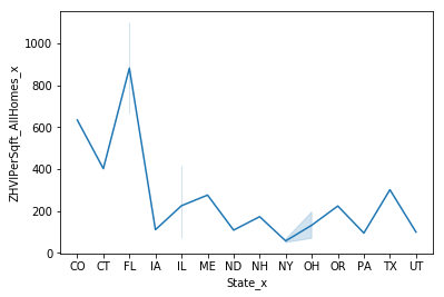
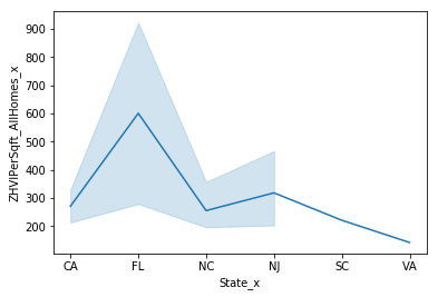
sns.lineplot(x="State_x", y="ZHVIPerSqft_AllHomes_x",data=comparison_a_graph)
<matplotlib.axes._subplots.AxesSubplot at 0x1a31652cc0>

test_graph = sns.barplot(x="State_x", y="ZHVIPerSqft_AllHomes_x", data=comparison_a_graph)
test_graph.set_xticklabels(max_graph.get_xticklabels(), rotation=90,size=7)
[Text(0, 0, 'VA'),
 Text(0, 0, 'CO'),
 Text(0, 0, 'CA'),
 Text(0, 0, 'TN'),
 Text(0, 0, 'DE')]

comparison_a.iloc[comparison_a["Dif"].idxmin()]
Date_x                          2017-05-31 00:00:00
RegionName                fisher_islandmiami_dadefl
ZHVIPerSqft_AllHomes_x                         1098
Year_x                                         2017
Month_x                                           5
City_x                                Fisher Island
County_x                                 Miami-Dade
State_x                                          FL
Date_y                          2016-05-31 00:00:00
ZHVIPerSqft_AllHomes_y                         1183
Year_y                                         2016
Month_y                                           5
City_y                                Fisher Island
County_y                                 Miami-Dade
State_y                                          FL
Dif                                             -85
Name: 3426, dtype: object
comparison_a2_graph = comparison_a.sort_values(by=["Dif"],ascending=True)
comparison_a2_graph = comparison_a2_graph.head(20)
comparison_a2_graph
| Date_x | RegionName | ZHVIPerSqft_AllHomes_x | Year_x | Month_x | City_x | County_x | State_x | Date_y | ZHVIPerSqft_AllHomes_y | Year_y | Month_y | City_y | County_y | State_y | Dif | |
|---|---|---|---|---|---|---|---|---|---|---|---|---|---|---|---|---|
| 3426 | 2017-05-31 | fisher_islandmiami_dadefl | 1098.0 | 2017 | 5 | Fisher Island | Miami-Dade | FL | 2016-05-31 | 1183.0 | 2016 | 5 | Fisher Island | Miami-Dade | FL | -85.0 |
| 9735 | 2017-05-31 | snowmass_villagepitkinco | 634.0 | 2017 | 5 | Snowmass Village | Pitkin | CO | 2016-05-31 | 679.0 | 2016 | 5 | Snowmass Village | Pitkin | CO | -45.0 |
| 8269 | 2017-05-31 | piney_pointharristx | 307.0 | 2017 | 5 | Piney Point | Harris | TX | 2016-05-31 | 347.0 | 2016 | 5 | Piney Point | Harris | TX | -40.0 |
| 10845 | 2017-05-31 | town_of_scarboroughcumberlandme | 276.0 | 2017 | 5 | Town of Scarborough | Cumberland | ME | 2016-05-31 | 314.0 | 2016 | 5 | Town of Scarborough | Cumberland | ME | -38.0 |
| 9909 | 2017-05-31 | southside_placeharristx | 296.0 | 2017 | 5 | Southside Place | Harris | TX | 2016-05-31 | 329.0 | 2016 | 5 | Southside Place | Harris | TX | -33.0 |
| 4043 | 2017-05-31 | grand_forksgrand_forksnd | 109.0 | 2017 | 5 | Grand Forks | Grand Forks | ND | 2016-05-31 | 137.0 | 2016 | 5 | Grand Forks | Grand Forks | ND | -28.0 |
| 5249 | 2017-05-31 | key_biscaynemiami_dadefl | 664.0 | 2017 | 5 | Key Biscayne | Miami-Dade | FL | 2016-05-31 | 688.0 | 2016 | 5 | Key Biscayne | Miami-Dade | FL | -24.0 |
| 9009 | 2017-05-31 | rooseveltduchesneut | 100.0 | 2017 | 5 | Roosevelt | Duchesne | UT | 2016-05-31 | 120.0 | 2016 | 5 | Roosevelt | Duchesne | UT | -20.0 |
| 8558 | 2017-05-31 | prophetstownwhitesideil | 71.0 | 2017 | 5 | Prophetstown | Whiteside | IL | 2016-05-31 | 89.0 | 2016 | 5 | Prophetstown | Whiteside | IL | -18.0 |
| 5200 | 2017-05-31 | kenilworthcookil | 417.0 | 2017 | 5 | Kenilworth | Cook | IL | 2016-05-31 | 435.0 | 2016 | 5 | Kenilworth | Cook | IL | -18.0 |
| 11967 | 2017-05-31 | wiltonmuscatineia | 111.0 | 2017 | 5 | Wilton | Muscatine | IA | 2016-05-31 | 129.0 | 2016 | 5 | Wilton | Muscatine | IA | -18.0 |
| 8587 | 2017-05-31 | put_in_bayottawaoh | 195.0 | 2017 | 5 | Put in Bay | Ottawa | OH | 2016-05-31 | 213.0 | 2016 | 5 | Put in Bay | Ottawa | OH | -18.0 |
| 4695 | 2017-05-31 | holdernessgraftonnh | 173.0 | 2017 | 5 | Holderness | Grafton | NH | 2016-05-31 | 189.0 | 2016 | 5 | Holderness | Grafton | NH | -16.0 |
| 10537 | 2017-05-31 | town_of_almondalleganyny | 50.0 | 2017 | 5 | Town of Almond | Allegany | NY | 2016-05-31 | 65.0 | 2016 | 5 | Town of Almond | Allegany | NY | -15.0 |
| 11135 | 2017-05-31 | uticalickingoh | 70.0 | 2017 | 5 | Utica | Licking | OH | 2016-05-31 | 84.0 | 2016 | 5 | Utica | Licking | OH | -14.0 |
| 6540 | 2017-05-31 | mettawalakeil | 188.0 | 2017 | 5 | Mettawa | Lake | IL | 2016-05-31 | 202.0 | 2016 | 5 | Mettawa | Lake | IL | -14.0 |
| 10182 | 2017-05-31 | sugarcreek_townshiparmstrongpa | 95.0 | 2017 | 5 | Sugarcreek Township | Armstrong | PA | 2016-05-31 | 108.0 | 2016 | 5 | Sugarcreek Township | Armstrong | PA | -13.0 |
| 7127 | 2017-05-31 | nehalemtillamookor | 224.0 | 2017 | 5 | Nehalem | Tillamook | OR | 2016-05-31 | 237.0 | 2016 | 5 | Nehalem | Tillamook | OR | -13.0 |
| 11777 | 2017-05-31 | westportfairfieldct | 402.0 | 2017 | 5 | Westport | Fairfield | CT | 2016-05-31 | 415.0 | 2016 | 5 | Westport | Fairfield | CT | -13.0 |
| 9102 | 2017-05-31 | rushfordalleganyny | 65.0 | 2017 | 5 | Rushford | Allegany | NY | 2016-05-31 | 78.0 | 2016 | 5 | Rushford | Allegany | NY | -13.0 |
comparison_a2_graph.to_csv("comparison_a2_graph.csv",encoding='utf-8', index=False)
sns.lineplot(x="State_x", y="ZHVIPerSqft_AllHomes_x",data=comparison_a2_graph)
<matplotlib.axes._subplots.AxesSubplot at 0x1a354ae780>

sqft_2017b = sqft_2017
sqft_2012a = q3.loc[q3['Year']==2012]
sqft_2012 = sqft_2012a.loc[sqft_2012a['Month']==5]
comparison_b = pd.merge(sqft_2017b,sqft_2012, on='RegionName')
#comparison_b = comparison_b[["RegionName_x","ZHVIPerSqft_AllHomes_x","Year_x","City","State_x","ZHVIPerSqft_AllHomes_y","Year_y"]]
comparison_b['Dif'] = comparison_b["ZHVIPerSqft_AllHomes_x"] - comparison_b["ZHVIPerSqft_AllHomes_y"]
#comparison_b.head()
comparison_b.iloc[comparison_b["Dif"].idxmax()]
Date_x                       2017-05-31 00:00:00
RegionName                palo_altosanta_claraca
ZHVIPerSqft_AllHomes_x                      1574
Year_x                                      2017
Month_x                                        5
City_x                                 Palo Alto
County_x                             Santa Clara
State_x                                       CA
Date_y                       2012-05-31 00:00:00
ZHVIPerSqft_AllHomes_y                       801
Year_y                                      2012
Month_y                                        5
City_y                                 Palo Alto
County_y                             Santa Clara
State_y                                       CA
Dif                                          773
Name: 7859, dtype: object
comparison_b_graph = comparison_b.sort_values(by=["Dif"],ascending=False)
comparison_b_graph = comparison_b_graph.head(20)
comparison_b_graph
| Date_x | RegionName | ZHVIPerSqft_AllHomes_x | Year_x | Month_x | City_x | County_x | State_x | Date_y | ZHVIPerSqft_AllHomes_y | Year_y | Month_y | City_y | County_y | State_y | Dif | |
|---|---|---|---|---|---|---|---|---|---|---|---|---|---|---|---|---|
| 7859 | 2017-05-31 | palo_altosanta_claraca | 1574.0 | 2017 | 5 | Palo Alto | Santa Clara | CA | 2012-05-31 | 801.0 | 2012 | 5 | Palo Alto | Santa Clara | CA | 773.0 |
| 349 | 2017-05-31 | athertonsan_mateoca | 1746.0 | 2017 | 5 | Atherton | San Mateo | CA | 2012-05-31 | 977.0 | 2012 | 5 | Atherton | San Mateo | CA | 769.0 |
| 9980 | 2017-05-31 | stinson_beachmarinca | 1709.0 | 2017 | 5 | Stinson Beach | Marin | CA | 2012-05-31 | 1040.0 | 2012 | 5 | Stinson Beach | Marin | CA | 669.0 |
| 9919 | 2017-05-31 | stanfordsanta_claraca | 1286.0 | 2017 | 5 | Stanford | Santa Clara | CA | 2012-05-31 | 715.0 | 2012 | 5 | Stanford | Santa Clara | CA | 571.0 |
| 5896 | 2017-05-31 | los_altossanta_claraca | 1271.0 | 2017 | 5 | Los Altos | Santa Clara | CA | 2012-05-31 | 724.0 | 2012 | 5 | Los Altos | Santa Clara | CA | 547.0 |
| 5895 | 2017-05-31 | los_altos_hillssanta_claraca | 1336.0 | 2017 | 5 | Los Altos Hills | Santa Clara | CA | 2012-05-31 | 797.0 | 2012 | 5 | Los Altos Hills | Santa Clara | CA | 539.0 |
| 11973 | 2017-05-31 | woodsidesan_mateoca | 1375.0 | 2017 | 5 | Woodside | San Mateo | CA | 2012-05-31 | 838.0 | 2012 | 5 | Woodside | San Mateo | CA | 537.0 |
| 8386 | 2017-05-31 | portola_valleysan_mateoca | 1376.0 | 2017 | 5 | Portola Valley | San Mateo | CA | 2012-05-31 | 864.0 | 2012 | 5 | Portola Valley | San Mateo | CA | 512.0 |
| 6428 | 2017-05-31 | menlo_parksan_mateoca | 1175.0 | 2017 | 5 | Menlo Park | San Mateo | CA | 2012-05-31 | 681.0 | 2012 | 5 | Menlo Park | San Mateo | CA | 494.0 |
| 6920 | 2017-05-31 | mountain_viewsanta_claraca | 995.0 | 2017 | 5 | Mountain View | Santa Clara | CA | 2012-05-31 | 501.0 | 2012 | 5 | Mountain View | Santa Clara | CA | 494.0 |
| 4604 | 2017-05-31 | hillsboroughsan_mateoca | 1224.0 | 2017 | 5 | Hillsborough | San Mateo | CA | 2012-05-31 | 745.0 | 2012 | 5 | Hillsborough | San Mateo | CA | 479.0 |
| 10120 | 2017-05-31 | sunnyvalesanta_claraca | 940.0 | 2017 | 5 | Sunnyvale | Santa Clara | CA | 2012-05-31 | 466.0 | 2012 | 5 | Sunnyvale | Santa Clara | CA | 474.0 |
| 7338 | 2017-05-31 | north_fair_oakssan_mateoca | 821.0 | 2017 | 5 | North Fair Oaks | San Mateo | CA | 2012-05-31 | 354.0 | 2012 | 5 | North Fair Oaks | San Mateo | CA | 467.0 |
| 817 | 2017-05-31 | beverly_hillslos_angelesca | 1140.0 | 2017 | 5 | Beverly Hills | Los Angeles | CA | 2012-05-31 | 677.0 | 2012 | 5 | Beverly Hills | Los Angeles | CA | 463.0 |
| 2868 | 2017-05-31 | east_palo_altosan_mateoca | 689.0 | 2017 | 5 | East Palo Alto | San Mateo | CA | 2012-05-31 | 250.0 | 2012 | 5 | East Palo Alto | San Mateo | CA | 439.0 |
| 713 | 2017-05-31 | belvederemarinca | 1333.0 | 2017 | 5 | Belvedere | Marin | CA | 2012-05-31 | 896.0 | 2012 | 5 | Belvedere | Marin | CA | 437.0 |
| 6124 | 2017-05-31 | manhattan_beachlos_angelesca | 1039.0 | 2017 | 5 | Manhattan Beach | Los Angeles | CA | 2012-05-31 | 605.0 | 2012 | 5 | Manhattan Beach | Los Angeles | CA | 434.0 |
| 2364 | 2017-05-31 | cupertinosanta_claraca | 1009.0 | 2017 | 5 | Cupertino | Santa Clara | CA | 2012-05-31 | 576.0 | 2012 | 5 | Cupertino | Santa Clara | CA | 433.0 |
| 4582 | 2017-05-31 | highlands_baywood_parksan_mateoca | 963.0 | 2017 | 5 | Highlands-Baywood Park | San Mateo | CA | 2012-05-31 | 533.0 | 2012 | 5 | Highlands-Baywood Park | San Mateo | CA | 430.0 |
| 9040 | 2017-05-31 | sag_harborsuffolkny | 1029.0 | 2017 | 5 | Sag Harbor | Suffolk | NY | 2012-05-31 | 604.0 | 2012 | 5 | Sag Harbor | Suffolk | NY | 425.0 |
comparison_b_graph.to_csv("comparison_b_graph.csv",encoding='utf-8', index=False)
comparison_b2_graph = comparison_b.sort_values(by=["Dif"],ascending=True)
comparison_b2_graph = comparison_b2_graph.head(20)
comparison_b2_graph
| Date_x | RegionName | ZHVIPerSqft_AllHomes_x | Year_x | Month_x | City_x | County_x | State_x | Date_y | ZHVIPerSqft_AllHomes_y | Year_y | Month_y | City_y | County_y | State_y | Dif | |
|---|---|---|---|---|---|---|---|---|---|---|---|---|---|---|---|---|
| 8903 | 2017-05-31 | rooseveltduchesneut | 100.0 | 2017 | 5 | Roosevelt | Duchesne | UT | 2012-05-31 | 160.0 | 2012 | 5 | Roosevelt | Duchesne | UT | -60.0 |
| 9792 | 2017-05-31 | southportlincolnme | 302.0 | 2017 | 5 | Southport | Lincoln | ME | 2012-05-31 | 331.0 | 2012 | 5 | Southport | Lincoln | ME | -29.0 |
| 11102 | 2017-05-31 | versaillesdarkeoh | 83.0 | 2017 | 5 | Versailles | Darke | OH | 2012-05-31 | 106.0 | 2012 | 5 | Versailles | Darke | OH | -23.0 |
| 4121 | 2017-05-31 | greenvilledarkeoh | 69.0 | 2017 | 5 | Greenville | Darke | OH | 2012-05-31 | 90.0 | 2012 | 5 | Greenville | Darke | OH | -21.0 |
| 2606 | 2017-05-31 | dickinsonstarknd | 172.0 | 2017 | 5 | Dickinson | Stark | ND | 2012-05-31 | 193.0 | 2012 | 5 | Dickinson | Stark | ND | -21.0 |
| 258 | 2017-05-31 | arcanumdarkeoh | 70.0 | 2017 | 5 | Arcanum | Darke | OH | 2012-05-31 | 90.0 | 2012 | 5 | Arcanum | Darke | OH | -20.0 |
| 11080 | 2017-05-31 | ventnor_cityatlanticnj | 164.0 | 2017 | 5 | Ventnor City | Atlantic | NJ | 2012-05-31 | 181.0 | 2012 | 5 | Ventnor City | Atlantic | NJ | -17.0 |
| 5747 | 2017-05-31 | linwooddelawarepa | 64.0 | 2017 | 5 | Linwood | Delaware | PA | 2012-05-31 | 79.0 | 2012 | 5 | Linwood | Delaware | PA | -15.0 |
| 3707 | 2017-05-31 | galenajo_daviessil | 90.0 | 2017 | 5 | Galena | Jo Daviess | IL | 2012-05-31 | 104.0 | 2012 | 5 | Galena | Jo Daviess | IL | -14.0 |
| 5090 | 2017-05-31 | kankakeekankakeeil | 58.0 | 2017 | 5 | Kankakee | Kankakee | IL | 2012-05-31 | 72.0 | 2012 | 5 | Kankakee | Kankakee | IL | -14.0 |
| 1027 | 2017-05-31 | bradleykankakeeil | 80.0 | 2017 | 5 | Bradley | Kankakee | IL | 2012-05-31 | 93.0 | 2012 | 5 | Bradley | Kankakee | IL | -13.0 |
| 910 | 2017-05-31 | blue_earthfaribaultmn | 91.0 | 2017 | 5 | Blue Earth | Faribault | MN | 2012-05-31 | 104.0 | 2012 | 5 | Blue Earth | Faribault | MN | -13.0 |
| 5973 | 2017-05-31 | lumbertonlamarms | 59.0 | 2017 | 5 | Lumberton | Lamar | MS | 2012-05-31 | 72.0 | 2012 | 5 | Lumberton | Lamar | MS | -13.0 |
| 8347 | 2017-05-31 | port_isabelcamerontx | 137.0 | 2017 | 5 | Port Isabel | Cameron | TX | 2012-05-31 | 150.0 | 2012 | 5 | Port Isabel | Cameron | TX | -13.0 |
| 201 | 2017-05-31 | andrewsandrewstx | 96.0 | 2017 | 5 | Andrews | Andrews | TX | 2012-05-31 | 109.0 | 2012 | 5 | Andrews | Andrews | TX | -13.0 |
| 9073 | 2017-05-31 | saint_henrymerceroh | 104.0 | 2017 | 5 | Saint Henry | Mercer | OH | 2012-05-31 | 116.0 | 2012 | 5 | Saint Henry | Mercer | OH | -12.0 |
| 11023 | 2017-05-31 | vails_gateorangeny | 133.0 | 2017 | 5 | Vails Gate | Orange | NY | 2012-05-31 | 145.0 | 2012 | 5 | Vails Gate | Orange | NY | -12.0 |
| 5745 | 2017-05-31 | linwoodatlanticnj | 121.0 | 2017 | 5 | Linwood | Atlantic | NJ | 2012-05-31 | 133.0 | 2012 | 5 | Linwood | Atlantic | NJ | -12.0 |
| 2191 | 2017-05-31 | corollacurritucknc | 185.0 | 2017 | 5 | Corolla | Currituck | NC | 2012-05-31 | 197.0 | 2012 | 5 | Corolla | Currituck | NC | -12.0 |
| 10811 | 2017-05-31 | trainerdelawarepa | 71.0 | 2017 | 5 | Trainer | Delaware | PA | 2012-05-31 | 82.0 | 2012 | 5 | Trainer | Delaware | PA | -11.0 |
comparison_b2_graph.to_csv("comparison_b2_graph.csv",encoding='utf-8', index=False)
sqft_2017c = sqft_2017
sqft_2007a = q3.loc[q3['Year']==2007]
sqft_2007 = sqft_2007a.loc[sqft_2007a['Month']==5]
comparison_c = pd.merge(sqft_2017c,sqft_2007, on='RegionName')
#comparison_c = comparison_c[["RegionName_x","ZHVIPerSqft_AllHomes_x","Year_x","City","State_x","ZHVIPerSqft_AllHomes_y","Year_y"]]
comparison_c['Dif'] = comparison_c["ZHVIPerSqft_AllHomes_x"] - comparison_c["ZHVIPerSqft_AllHomes_y"]
comparison_c.iloc[comparison_c["Dif"].idxmax()]
Date_x                       2017-05-31 00:00:00
RegionName                palo_altosanta_claraca
ZHVIPerSqft_AllHomes_x                      1574
Year_x                                      2017
Month_x                                        5
City_x                                 Palo Alto
County_x                             Santa Clara
State_x                                       CA
Date_y                       2007-05-31 00:00:00
ZHVIPerSqft_AllHomes_y                       753
Year_y                                      2007
Month_y                                        5
City_y                                 Palo Alto
County_y                             Santa Clara
State_y                                       CA
Dif                                          821
Name: 7262, dtype: object
comparison_c_graph = comparison_c.sort_values(by=["Dif"],ascending=False)
comparison_c_graph = comparison_c_graph.head(20)
comparison_c_graph
| Date_x | RegionName | ZHVIPerSqft_AllHomes_x | Year_x | Month_x | City_x | County_x | State_x | Date_y | ZHVIPerSqft_AllHomes_y | Year_y | Month_y | City_y | County_y | State_y | Dif | |
|---|---|---|---|---|---|---|---|---|---|---|---|---|---|---|---|---|
| 7262 | 2017-05-31 | palo_altosanta_claraca | 1574.0 | 2017 | 5 | Palo Alto | Santa Clara | CA | 2007-05-31 | 753.0 | 2007 | 5 | Palo Alto | Santa Clara | CA | 821.0 |
| 320 | 2017-05-31 | athertonsan_mateoca | 1746.0 | 2017 | 5 | Atherton | San Mateo | CA | 2007-05-31 | 1058.0 | 2007 | 5 | Atherton | San Mateo | CA | 688.0 |
| 9242 | 2017-05-31 | stinson_beachmarinca | 1709.0 | 2017 | 5 | Stinson Beach | Marin | CA | 2007-05-31 | 1060.0 | 2007 | 5 | Stinson Beach | Marin | CA | 649.0 |
| 5440 | 2017-05-31 | los_altossanta_claraca | 1271.0 | 2017 | 5 | Los Altos | Santa Clara | CA | 2007-05-31 | 725.0 | 2007 | 5 | Los Altos | Santa Clara | CA | 546.0 |
| 9185 | 2017-05-31 | stanfordsanta_claraca | 1286.0 | 2017 | 5 | Stanford | Santa Clara | CA | 2007-05-31 | 751.0 | 2007 | 5 | Stanford | Santa Clara | CA | 535.0 |
| 5439 | 2017-05-31 | los_altos_hillssanta_claraca | 1336.0 | 2017 | 5 | Los Altos Hills | Santa Clara | CA | 2007-05-31 | 871.0 | 2007 | 5 | Los Altos Hills | Santa Clara | CA | 465.0 |
| 6386 | 2017-05-31 | mountain_viewsanta_claraca | 995.0 | 2017 | 5 | Mountain View | Santa Clara | CA | 2007-05-31 | 546.0 | 2007 | 5 | Mountain View | Santa Clara | CA | 449.0 |
| 5925 | 2017-05-31 | menlo_parksan_mateoca | 1175.0 | 2017 | 5 | Menlo Park | San Mateo | CA | 2007-05-31 | 728.0 | 2007 | 5 | Menlo Park | San Mateo | CA | 447.0 |
| 11098 | 2017-05-31 | woodsidesan_mateoca | 1375.0 | 2017 | 5 | Woodside | San Mateo | CA | 2007-05-31 | 958.0 | 2007 | 5 | Woodside | San Mateo | CA | 417.0 |
| 2169 | 2017-05-31 | cupertinosanta_claraca | 1009.0 | 2017 | 5 | Cupertino | Santa Clara | CA | 2007-05-31 | 594.0 | 2007 | 5 | Cupertino | Santa Clara | CA | 415.0 |
| 4218 | 2017-05-31 | highlands_baywood_parksan_mateoca | 963.0 | 2017 | 5 | Highlands-Baywood Park | San Mateo | CA | 2007-05-31 | 550.0 | 2007 | 5 | Highlands-Baywood Park | San Mateo | CA | 413.0 |
| 9370 | 2017-05-31 | sunnyvalesanta_claraca | 940.0 | 2017 | 5 | Sunnyvale | Santa Clara | CA | 2007-05-31 | 534.0 | 2007 | 5 | Sunnyvale | Santa Clara | CA | 406.0 |
| 1164 | 2017-05-31 | burlingamesan_mateoca | 1034.0 | 2017 | 5 | Burlingame | San Mateo | CA | 2007-05-31 | 640.0 | 2007 | 5 | Burlingame | San Mateo | CA | 394.0 |
| 7754 | 2017-05-31 | portola_valleysan_mateoca | 1376.0 | 2017 | 5 | Portola Valley | San Mateo | CA | 2007-05-31 | 987.0 | 2007 | 5 | Portola Valley | San Mateo | CA | 389.0 |
| 8359 | 2017-05-31 | sag_harborsuffolkny | 1029.0 | 2017 | 5 | Sag Harbor | Suffolk | NY | 2007-05-31 | 647.0 | 2007 | 5 | Sag Harbor | Suffolk | NY | 382.0 |
| 650 | 2017-05-31 | belvederemarinca | 1333.0 | 2017 | 5 | Belvedere | Marin | CA | 2007-05-31 | 958.0 | 2007 | 5 | Belvedere | Marin | CA | 375.0 |
| 642 | 2017-05-31 | belmontsan_mateoca | 907.0 | 2017 | 5 | Belmont | San Mateo | CA | 2007-05-31 | 537.0 | 2007 | 5 | Belmont | San Mateo | CA | 370.0 |
| 8564 | 2017-05-31 | saratogasanta_claraca | 1025.0 | 2017 | 5 | Saratoga | Santa Clara | CA | 2007-05-31 | 680.0 | 2007 | 5 | Saratoga | Santa Clara | CA | 345.0 |
| 741 | 2017-05-31 | beverly_hillslos_angelesca | 1140.0 | 2017 | 5 | Beverly Hills | Los Angeles | CA | 2007-05-31 | 797.0 | 2007 | 5 | Beverly Hills | Los Angeles | CA | 343.0 |
| 8471 | 2017-05-31 | san_carlossan_mateoca | 929.0 | 2017 | 5 | San Carlos | San Mateo | CA | 2007-05-31 | 594.0 | 2007 | 5 | San Carlos | San Mateo | CA | 335.0 |
comparison_c_graph.to_csv("comparison_c_graph.csv",encoding='utf-8', index=False)
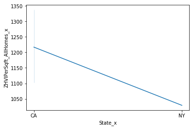
sns.lineplot(x="State_x", y="ZHVIPerSqft_AllHomes_x",data=comparison_c_graph)
<matplotlib.axes._subplots.AxesSubplot at 0x1a357b9c50>

comparison_c2_graph = comparison_c.sort_values(by=["Dif"],ascending=True)
comparison_c2_graph = comparison_c2_graph.head(21)
comparison_c2_graph
| Date_x | RegionName | ZHVIPerSqft_AllHomes_x | Year_x | Month_x | City_x | County_x | State_x | Date_y | ZHVIPerSqft_AllHomes_y | Year_y | Month_y | City_y | County_y | State_y | Dif | |
|---|---|---|---|---|---|---|---|---|---|---|---|---|---|---|---|---|
| 4844 | 2017-05-31 | kirkwoodalpineca | 283.0 | 2017 | 5 | Kirkwood | Alpine | CA | 2007-05-31 | 528.0 | 2007 | 5 | Kirkwood | Alpine | CA | -245.0 |
| 11130 | 2017-05-31 | wrightsville_beachnew_hanovernc | 555.0 | 2017 | 5 | Wrightsville Beach | New Hanover | NC | 2007-05-31 | 758.0 | 2007 | 5 | Wrightsville Beach | New Hanover | NC | -203.0 |
| 4678 | 2017-05-31 | jupiter_islandmartinfl | 923.0 | 2017 | 5 | Jupiter Island | Martin | FL | 2007-05-31 | 1114.0 | 2007 | 5 | Jupiter Island | Martin | FL | -191.0 |
| 940 | 2017-05-31 | bradleysan_luis_obispoca | 246.0 | 2017 | 5 | Bradley | San Luis Obispo | CA | 2007-05-31 | 426.0 | 2007 | 5 | Bradley | San Luis Obispo | CA | -180.0 |
| 2741 | 2017-05-31 | edisto_beachcolletonsc | 221.0 | 2017 | 5 | Edisto Beach | Colleton | SC | 2007-05-31 | 391.0 | 2007 | 5 | Edisto Beach | Colleton | SC | -170.0 |
| 4491 | 2017-05-31 | indian_beachcarteretnc | 221.0 | 2017 | 5 | Indian Beach | Carteret | NC | 2007-05-31 | 389.0 | 2007 | 5 | Indian Beach | Carteret | NC | -168.0 |
| 326 | 2017-05-31 | atlantic_beachcarteretnc | 205.0 | 2017 | 5 | Atlantic Beach | Carteret | NC | 2007-05-31 | 371.0 | 2007 | 5 | Atlantic Beach | Carteret | NC | -166.0 |
| 5630 | 2017-05-31 | mammoth_lakesmonoca | 296.0 | 2017 | 5 | Mammoth Lakes | Mono | CA | 2007-05-31 | 447.0 | 2007 | 5 | Mammoth Lakes | Mono | CA | -151.0 |
| 10797 | 2017-05-31 | westwoodplumasca | 167.0 | 2017 | 5 | Westwood | Plumas | CA | 2007-05-31 | 316.0 | 2007 | 5 | Westwood | Plumas | CA | -149.0 |
| 6988 | 2017-05-31 | ocean_isle_beachbrunswicknc | 193.0 | 2017 | 5 | Ocean Isle Beach | Brunswick | NC | 2007-05-31 | 338.0 | 2007 | 5 | Ocean Isle Beach | Brunswick | NC | -145.0 |
| 7538 | 2017-05-31 | pine_knoll_shorescarteretnc | 196.0 | 2017 | 5 | Pine Knoll Shores | Carteret | NC | 2007-05-31 | 336.0 | 2007 | 5 | Pine Knoll Shores | Carteret | NC | -140.0 |
| 2018 | 2017-05-31 | corollacurritucknc | 185.0 | 2017 | 5 | Corolla | Currituck | NC | 2007-05-31 | 323.0 | 2007 | 5 | Corolla | Currituck | NC | -138.0 |
| 7134 | 2017-05-31 | ortley_beachoceannj | 285.0 | 2017 | 5 | Ortley Beach | Ocean | NJ | 2007-05-31 | 419.0 | 2007 | 5 | Ortley Beach | Ocean | NJ | -134.0 |
| 2099 | 2017-05-31 | crescent_beachsaint_johnsfl | 279.0 | 2017 | 5 | Crescent Beach | Saint Johns | FL | 2007-05-31 | 411.0 | 2007 | 5 | Crescent Beach | Saint Johns | FL | -132.0 |
| 1014 | 2017-05-31 | brigantineatlanticnj | 203.0 | 2017 | 5 | Brigantine | Atlantic | NJ | 2007-05-31 | 335.0 | 2007 | 5 | Brigantine | Atlantic | NJ | -132.0 |
| 8241 | 2017-05-31 | roselandnelsonva | 142.0 | 2017 | 5 | Roseland | Nelson | VA | 2007-05-31 | 265.0 | 2007 | 5 | Roseland | Nelson | VA | -123.0 |
| 3347 | 2017-05-31 | freedomsanta_cruzca | 356.0 | 2017 | 5 | Freedom | Santa Cruz | CA | 2007-05-31 | 478.0 | 2007 | 5 | Freedom | Santa Cruz | CA | -122.0 |
| 8657 | 2017-05-31 | seasidemontereyca | 393.0 | 2017 | 5 | Seaside | Monterey | CA | 2007-05-31 | 513.0 | 2007 | 5 | Seaside | Monterey | CA | -120.0 |
| 2869 | 2017-05-31 | emerald_islecarteretnc | 232.0 | 2017 | 5 | Emerald Isle | Carteret | NC | 2007-05-31 | 350.0 | 2007 | 5 | Emerald Isle | Carteret | NC | -118.0 |
| 5415 | 2017-05-31 | longportatlanticnj | 467.0 | 2017 | 5 | Longport | Atlantic | NJ | 2007-05-31 | 585.0 | 2007 | 5 | Longport | Atlantic | NJ | -118.0 |
| 1607 | 2017-05-31 | chesterplumasca | 155.0 | 2017 | 5 | Chester | Plumas | CA | 2007-05-31 | 272.0 | 2007 | 5 | Chester | Plumas | CA | -117.0 |
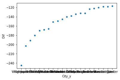
sns.scatterplot(y="Dif", x="City_y", data=comparison_c2_graph)
<matplotlib.axes._subplots.AxesSubplot at 0x1a3898f7b8>

sns.lineplot(x="State_x", y="ZHVIPerSqft_AllHomes_x",data=comparison_c2_graph)
<matplotlib.axes._subplots.AxesSubplot at 0x1a35799780>

comparison_c2_graph.to_csv("comparison_c2_graph.csv",encoding='utf-8', index=False)
QUESTION 4: For a city of choice, (most likely Ann Arbor) have prices for each size of home changed in similar amounts over the course of the datasets recordings or are there some sizes that are more affordable or less affordable within the city?
Calculate the mean increase for each type of home (1 bedroom, 2 bedroom, etc.) in Ann Arbor. Calculate the average price change for each of these types of homes year to year. Compare the average price change, is it similar or different? I think a histogram will be a good way to visualize this, but I could potentially create a story in Tableau which might walk the viewer through the information.
q4 = city_state_data
q4 = q4[["Date","Year","Month","RegionName","ZHVI_1bedroom","ZHVI_2bedroom","ZHVI_3bedroom","ZHVI_4bedroom","ZHVI_5BedroomOrMore","ZHVIPerSqft_AllHomes","ZHVI_BottomTier","ZHVI_MiddleTier","ZHVI_SingleFamilyResidence","ZHVI_TopTier","State","County","City"]]
q4 = q4.dropna()
q4.head()
| Date | Year | Month | RegionName | ZHVI_1bedroom | ZHVI_2bedroom | ZHVI_3bedroom | ZHVI_4bedroom | ZHVI_5BedroomOrMore | ZHVIPerSqft_AllHomes | ZHVI_BottomTier | ZHVI_MiddleTier | ZHVI_SingleFamilyResidence | ZHVI_TopTier | State | County | City | |
|---|---|---|---|---|---|---|---|---|---|---|---|---|---|---|---|---|---|
| 10 | 1996-04-30 | 1996 | 4 | abingtonmontgomerypa | 47500.0 | 102200.0 | 122000.0 | 157600.0 | 219000.0 | 78.0 | 102000.0 | 128700.0 | 130900.0 | 189400.0 | PA | Montgomery | Abington |
| 18 | 1996-04-30 | 1996 | 4 | actonmiddlesexma | 52400.0 | 122200.0 | 212500.0 | 288100.0 | 325500.0 | 118.0 | 128200.0 | 230500.0 | 253900.0 | 330100.0 | MA | Middlesex | Acton |
| 21 | 1996-04-30 | 1996 | 4 | acworthcobbga | 62200.0 | 75500.0 | 100800.0 | 155900.0 | 201300.0 | 60.0 | 83900.0 | 112900.0 | 114800.0 | 174000.0 | GA | Cobb | Acworth |
| 44 | 1996-04-30 | 1996 | 4 | agawamhampdenma | 35800.0 | 82100.0 | 107400.0 | 114100.0 | 127300.0 | 71.0 | 68600.0 | 101500.0 | 106800.0 | 124700.0 | MA | Hampden | Agawam |
| 55 | 1996-04-30 | 1996 | 4 | akronsummitoh | 41600.0 | 49100.0 | 59500.0 | 70000.0 | 74900.0 | 49.0 | 42800.0 | 57100.0 | 56300.0 | 88000.0 | OH | Summit | Akron |
ann_arbor = q4.loc[q4["RegionName"]=="ann_arborwashtenawmi"]
ann_arbor.head()
| Date | Year | Month | RegionName | ZHVI_1bedroom | ZHVI_2bedroom | ZHVI_3bedroom | ZHVI_4bedroom | ZHVI_5BedroomOrMore | ZHVIPerSqft_AllHomes | ZHVI_BottomTier | ZHVI_MiddleTier | ZHVI_SingleFamilyResidence | ZHVI_TopTier | State | County | City | |
|---|---|---|---|---|---|---|---|---|---|---|---|---|---|---|---|---|---|
| 209 | 1996-04-30 | 1996 | 4 | ann_arborwashtenawmi | 90300.0 | 107300.0 | 129000.0 | 188500.0 | 220200.0 | 95.0 | 106900.0 | 152000.0 | 157300.0 | 248200.0 | MI | Washtenaw | Ann Arbor |
| 11639 | 1996-05-31 | 1996 | 5 | ann_arborwashtenawmi | 87500.0 | 107500.0 | 130400.0 | 188600.0 | 219300.0 | 96.0 | 107900.0 | 153100.0 | 158500.0 | 249500.0 | MI | Washtenaw | Ann Arbor |
| 23211 | 1996-06-30 | 1996 | 6 | ann_arborwashtenawmi | 84100.0 | 107700.0 | 131500.0 | 188800.0 | 220700.0 | 97.0 | 108300.0 | 154200.0 | 159700.0 | 250900.0 | MI | Washtenaw | Ann Arbor |
| 34842 | 1996-07-31 | 1996 | 7 | ann_arborwashtenawmi | 81100.0 | 108600.0 | 132200.0 | 189100.0 | 222600.0 | 97.0 | 108900.0 | 154900.0 | 160300.0 | 251100.0 | MI | Washtenaw | Ann Arbor |
| 46479 | 1996-08-31 | 1996 | 8 | ann_arborwashtenawmi | 80700.0 | 109200.0 | 133200.0 | 189500.0 | 224800.0 | 97.0 | 109300.0 | 155300.0 | 160500.0 | 251500.0 | MI | Washtenaw | Ann Arbor |
ann_arbor2017 = ann_arbor.loc[ann_arbor["Year"]==2017]
ann_arbor2017["ZHVI_1bedroom"].median()
171350.0
ann_arbor2017["ZHVI_2bedroom"].median()
233000.0
ann_arbor2017["ZHVI_3bedroom"].median()
303150.0
ann_arbor2017["ZHVI_4bedroom"].median()
408050.0
ann_arbor2017["ZHVI_5BedroomOrMore"].median()
568850.0
ann_arbor2012 = ann_arbor.loc[ann_arbor["Year"]==2012]
ann_arbor2012["ZHVI_1bedroom"].median()
142800.0
ann_arbor2012["ZHVI_2bedroom"].median()
157750.0
ann_arbor2012["ZHVI_3bedroom"].median()
204450.0
ann_arbor2012["ZHVI_4bedroom"].median()
279500.0
ann_arbor2012["ZHVI_5BedroomOrMore"].median()
365800.0
ann_arbor2007 = ann_arbor.loc[ann_arbor["Year"]==2007]
ann_arbor2007["ZHVI_1bedroom"].median()
160400.0
ann_arbor2007["ZHVI_2bedroom"].median()
173050.0
ann_arbor2007["ZHVI_3bedroom"].median()
220000.0
ann_arbor2007["ZHVI_4bedroom"].median()
295500.0
ann_arbor2007["ZHVI_5BedroomOrMore"].median()
403150.0
ann_arbor2002 = ann_arbor.loc[ann_arbor["Year"]==2002]
ann_arbor2002["ZHVI_1bedroom"].median()
131750.0
ann_arbor2002["ZHVI_2bedroom"].median()
173650.0
ann_arbor2002["ZHVI_3bedroom"].median()
219950.0
ann_arbor2002["ZHVI_4bedroom"].median()
299700.0
ann_arbor2002["ZHVI_5BedroomOrMore"].median()
376850.0
QUESTION 5: (Extra) Determine which cities are likely to experience an increase in housing prices in the coming years.
(Extra) Use machine learning regression to determine which city is likely to have the largest price increase over the coming 1, 5 and 10 years. (Where does it make sense to invest?) Plot the results in a scatterplot with seaborn?
q5 = city_state_data
len(q5)
3762566
q5 = q5.loc[q5["State"]=='MI']
q5 = q5[["Date","Year","Month","RegionName","ZHVI_1bedroom","ZHVI_2bedroom","ZHVI_3bedroom","ZHVI_4bedroom","ZHVI_5BedroomOrMore","ZHVIPerSqft_AllHomes","ZHVI_BottomTier","ZHVI_MiddleTier","ZHVI_SingleFamilyResidence","ZHVI_TopTier","State","County","City"]]
q5 = q5.dropna()
q5.head()
| Date | Year | Month | RegionName | ZHVI_1bedroom | ZHVI_2bedroom | ZHVI_3bedroom | ZHVI_4bedroom | ZHVI_5BedroomOrMore | ZHVIPerSqft_AllHomes | ZHVI_BottomTier | ZHVI_MiddleTier | ZHVI_SingleFamilyResidence | ZHVI_TopTier | State | County | City | |
|---|---|---|---|---|---|---|---|---|---|---|---|---|---|---|---|---|---|
| 209 | 1996-04-30 | 1996 | 4 | ann_arborwashtenawmi | 90300.0 | 107300.0 | 129000.0 | 188500.0 | 220200.0 | 95.0 | 106900.0 | 152000.0 | 157300.0 | 248200.0 | MI | Washtenaw | Ann Arbor |
| 844 | 1996-04-30 | 1996 | 4 | bloomfield_hillsoaklandmi | 61500.0 | 117800.0 | 215800.0 | 315100.0 | 528700.0 | 108.0 | 170000.0 | 270000.0 | 299500.0 | 541900.0 | MI | Oakland | Bloomfield Hills |
| 3183 | 1996-04-30 | 1996 | 4 | ferndaleoaklandmi | 60700.0 | 63000.0 | 75800.0 | 95700.0 | 95100.0 | 71.0 | 58600.0 | 71000.0 | 71000.0 | 101200.0 | MI | Oakland | Ferndale |
| 3787 | 1996-04-30 | 1996 | 4 | grand_rapidskentmi | 71700.0 | 63100.0 | 71500.0 | 78300.0 | 86200.0 | 50.0 | 45900.0 | 65800.0 | 64300.0 | 105600.0 | MI | Kent | Grand Rapids |
| 4188 | 1996-04-30 | 1996 | 4 | hazel_parkoaklandmi | 42000.0 | 43800.0 | 54600.0 | 64100.0 | 71100.0 | 53.0 | 42300.0 | 51500.0 | 51500.0 | 64500.0 | MI | Oakland | Hazel Park |
len(q5)
4470
q5_2017 = q5.loc[q5["Year"]==2017]
q5_2017 = q5_2017.loc[q5_2017["Month"]==5]
#q5_2017.head()
q5_2015 = q5.loc[q5["Year"]==2015]
q5_2015 = q5_2015.loc[q5_2015["Month"]==5]
#q5_2017.head()
q5_a = pd.merge(q5_2017,q5_2015, on='RegionName')
q5_a = q5_a[["RegionName","Year_x","ZHVIPerSqft_AllHomes_x","Year_y","ZHVIPerSqft_AllHomes_y"]]
q5_a['Dif'] = q5_a["ZHVIPerSqft_AllHomes_x"] - q5_a["ZHVIPerSqft_AllHomes_y"]
q5_a
| RegionName | Year_x | ZHVIPerSqft_AllHomes_x | Year_y | ZHVIPerSqft_AllHomes_y | Dif | |
|---|---|---|---|---|---|---|
| 0 | ann_arborwashtenawmi | 2017 | 208.0 | 2015 | 184.0 | 24.0 |
| 1 | bloomfield_hillsoaklandmi | 2017 | 170.0 | 2015 | 161.0 | 9.0 |
| 2 | brightonlivingstonmi | 2017 | 143.0 | 2015 | 129.0 | 14.0 |
| 3 | detroitwaynemi | 2017 | 40.0 | 2015 | 34.0 | 6.0 |
| 4 | farmington_hillsoaklandmi | 2017 | 124.0 | 2015 | 113.0 | 11.0 |
| 5 | ferndaleoaklandmi | 2017 | 136.0 | 2015 | 108.0 | 28.0 |
| 6 | flintgeneseemi | 2017 | 40.0 | 2015 | 32.0 | 8.0 |
| 7 | grand_rapidskentmi | 2017 | 101.0 | 2015 | 79.0 | 22.0 |
| 8 | hazel_parkoaklandmi | 2017 | 67.0 | 2015 | 55.0 | 12.0 |
| 9 | hollandottawami | 2017 | 126.0 | 2015 | 107.0 | 19.0 |
| 10 | livoniawaynemi | 2017 | 134.0 | 2015 | 117.0 | 17.0 |
| 11 | milford_townshipoaklandmi | 2017 | 148.0 | 2015 | 134.0 | 14.0 |
| 12 | muskegon_townshipmuskegonmi | 2017 | 60.0 | 2015 | 51.0 | 9.0 |
| 13 | norton_shoresmuskegonmi | 2017 | 97.0 | 2015 | 82.0 | 15.0 |
| 14 | rochester_hillsoaklandmi | 2017 | 137.0 | 2015 | 126.0 | 11.0 |
| 15 | saginawsaginawmi | 2017 | 47.0 | 2015 | 43.0 | 4.0 |
| 16 | saint_clair_shoresmacombmi | 2017 | 116.0 | 2015 | 97.0 | 19.0 |
| 17 | south_lyonoaklandmi | 2017 | 145.0 | 2015 | 131.0 | 14.0 |
| 18 | troyoaklandmi | 2017 | 147.0 | 2015 | 133.0 | 14.0 |
| 19 | waterfordoaklandmi | 2017 | 113.0 | 2015 | 98.0 | 15.0 |
| 20 | west_bloomfieldoaklandmi | 2017 | 126.0 | 2015 | 116.0 | 10.0 |
len(q5_a)
21
q5_a['Label'] = np.where(q5_a['Dif']>=10 ,'yes','no')
q5_a
| RegionName | Year_x | ZHVIPerSqft_AllHomes_x | Year_y | ZHVIPerSqft_AllHomes_y | Dif | Label | |
|---|---|---|---|---|---|---|---|
| 0 | ann_arborwashtenawmi | 2017 | 208.0 | 2015 | 184.0 | 24.0 | yes |
| 1 | bloomfield_hillsoaklandmi | 2017 | 170.0 | 2015 | 161.0 | 9.0 | no |
| 2 | brightonlivingstonmi | 2017 | 143.0 | 2015 | 129.0 | 14.0 | yes |
| 3 | detroitwaynemi | 2017 | 40.0 | 2015 | 34.0 | 6.0 | no |
| 4 | farmington_hillsoaklandmi | 2017 | 124.0 | 2015 | 113.0 | 11.0 | yes |
| 5 | ferndaleoaklandmi | 2017 | 136.0 | 2015 | 108.0 | 28.0 | yes |
| 6 | flintgeneseemi | 2017 | 40.0 | 2015 | 32.0 | 8.0 | no |
| 7 | grand_rapidskentmi | 2017 | 101.0 | 2015 | 79.0 | 22.0 | yes |
| 8 | hazel_parkoaklandmi | 2017 | 67.0 | 2015 | 55.0 | 12.0 | yes |
| 9 | hollandottawami | 2017 | 126.0 | 2015 | 107.0 | 19.0 | yes |
| 10 | livoniawaynemi | 2017 | 134.0 | 2015 | 117.0 | 17.0 | yes |
| 11 | milford_townshipoaklandmi | 2017 | 148.0 | 2015 | 134.0 | 14.0 | yes |
| 12 | muskegon_townshipmuskegonmi | 2017 | 60.0 | 2015 | 51.0 | 9.0 | no |
| 13 | norton_shoresmuskegonmi | 2017 | 97.0 | 2015 | 82.0 | 15.0 | yes |
| 14 | rochester_hillsoaklandmi | 2017 | 137.0 | 2015 | 126.0 | 11.0 | yes |
| 15 | saginawsaginawmi | 2017 | 47.0 | 2015 | 43.0 | 4.0 | no |
| 16 | saint_clair_shoresmacombmi | 2017 | 116.0 | 2015 | 97.0 | 19.0 | yes |
| 17 | south_lyonoaklandmi | 2017 | 145.0 | 2015 | 131.0 | 14.0 | yes |
| 18 | troyoaklandmi | 2017 | 147.0 | 2015 | 133.0 | 14.0 | yes |
| 19 | waterfordoaklandmi | 2017 | 113.0 | 2015 | 98.0 | 15.0 | yes |
| 20 | west_bloomfieldoaklandmi | 2017 | 126.0 | 2015 | 116.0 | 10.0 | yes |
import numpy as np
import pandas as pd
import scipy as sp
import sklearn as sk
from sklearn.model_selection import train_test_split
from sklearn.model_selection import cross_val_score
import sklearn.ensemble as skens
import sklearn.metrics as skmetric
import sklearn.naive_bayes as sknb
import sklearn.tree as sktree
import matplotlib.pyplot as plt
%matplotlib inline
import seaborn as sns
sns.set(style='white', color_codes=True, font_scale=1.3)
import sklearn.externals.six as sksix
import IPython.display as ipd
from sklearn.model_selection import cross_val_score
from sklearn import metrics
import os
from sklearn.metrics import accuracy_score
df_q5_train,df_q5_test = train_test_split(q5_a, test_size=0.3)
gnb_model = sknb.GaussianNB()
# given sepal length, predict if setosa
gnb_model.fit(df_q5_train[['ZHVIPerSqft_AllHomes_y']],df_q5_train['Label'])
GaussianNB(priors=None, var_smoothing=1e-09)
y_pred = gnb_model.predict(df_q5_test[['ZHVIPerSqft_AllHomes_y']])
df_q5_test['predicted_nb'] = y_pred
/anaconda3/lib/python3.6/site-packages/ipykernel_launcher.py:2: SettingWithCopyWarning:
A value is trying to be set on a copy of a slice from a DataFrame.
Try using .loc[row_indexer,col_indexer] = value instead

See the caveats in the documentation: http://pandas.pydata.org/pandas-docs/stable/indexing.html#indexing-view-versus-copy
df_q5_test
| RegionName | Year_x | ZHVIPerSqft_AllHomes_x | Year_y | ZHVIPerSqft_AllHomes_y | Dif | Label | predicted_nb | |
|---|---|---|---|---|---|---|---|---|
| 9 | hollandottawami | 2017 | 126.0 | 2015 | 107.0 | 19.0 | yes | yes |
| 19 | waterfordoaklandmi | 2017 | 113.0 | 2015 | 98.0 | 15.0 | yes | yes |
| 20 | west_bloomfieldoaklandmi | 2017 | 126.0 | 2015 | 116.0 | 10.0 | yes | yes |
| 3 | detroitwaynemi | 2017 | 40.0 | 2015 | 34.0 | 6.0 | no | no |
| 16 | saint_clair_shoresmacombmi | 2017 | 116.0 | 2015 | 97.0 | 19.0 | yes | yes |
| 12 | muskegon_townshipmuskegonmi | 2017 | 60.0 | 2015 | 51.0 | 9.0 | no | no |
| 13 | norton_shoresmuskegonmi | 2017 | 97.0 | 2015 | 82.0 | 15.0 | yes | yes |
accuracy_score(df_q5_test["Label"], df_q5_test["predicted_nb"])
1.0
y_pred = gnb_model.predict(df_q5_test[['ZHVIPerSqft_AllHomes_x']])
df_q5_test['predicted_nb2'] = y_pred
/anaconda3/lib/python3.6/site-packages/ipykernel_launcher.py:2: SettingWithCopyWarning:
A value is trying to be set on a copy of a slice from a DataFrame.
Try using .loc[row_indexer,col_indexer] = value instead

See the caveats in the documentation: http://pandas.pydata.org/pandas-docs/stable/indexing.html#indexing-view-versus-copy
accuracy_score(df_q5_test["Label"], df_q5_test["predicted_nb2"])
0.8571428571428571
df_q5_test
| RegionName | Year_x | ZHVIPerSqft_AllHomes_x | Year_y | ZHVIPerSqft_AllHomes_y | Dif | Label | predicted_nb | predicted_nb2 | |
|---|---|---|---|---|---|---|---|---|---|
| 9 | hollandottawami | 2017 | 126.0 | 2015 | 107.0 | 19.0 | yes | yes | yes |
| 19 | waterfordoaklandmi | 2017 | 113.0 | 2015 | 98.0 | 15.0 | yes | yes | yes |
| 20 | west_bloomfieldoaklandmi | 2017 | 126.0 | 2015 | 116.0 | 10.0 | yes | yes | yes |
| 3 | detroitwaynemi | 2017 | 40.0 | 2015 | 34.0 | 6.0 | no | no | no |
| 16 | saint_clair_shoresmacombmi | 2017 | 116.0 | 2015 | 97.0 | 19.0 | yes | yes | yes |
| 12 | muskegon_townshipmuskegonmi | 2017 | 60.0 | 2015 | 51.0 | 9.0 | no | no | yes |
| 13 | norton_shoresmuskegonmi | 2017 | 97.0 | 2015 | 82.0 | 15.0 | yes | yes | yes |
Whole Country
q5_b = city_state_data
len(q5_b)
3762566
q5_b2 = q5_b[["Date","Year","Month","RegionName","ZHVI_1bedroom","ZHVI_2bedroom","ZHVI_3bedroom","ZHVI_4bedroom","ZHVI_5BedroomOrMore","ZHVIPerSqft_AllHomes","ZHVI_BottomTier","ZHVI_MiddleTier","ZHVI_SingleFamilyResidence","ZHVI_TopTier","State","County","City"]]
q5_b2 = q5_b2.dropna()
q5_b2.head()
| Date | Year | Month | RegionName | ZHVI_1bedroom | ZHVI_2bedroom | ZHVI_3bedroom | ZHVI_4bedroom | ZHVI_5BedroomOrMore | ZHVIPerSqft_AllHomes | ZHVI_BottomTier | ZHVI_MiddleTier | ZHVI_SingleFamilyResidence | ZHVI_TopTier | State | County | City | |
|---|---|---|---|---|---|---|---|---|---|---|---|---|---|---|---|---|---|
| 10 | 1996-04-30 | 1996 | 4 | abingtonmontgomerypa | 47500.0 | 102200.0 | 122000.0 | 157600.0 | 219000.0 | 78.0 | 102000.0 | 128700.0 | 130900.0 | 189400.0 | PA | Montgomery | Abington |
| 18 | 1996-04-30 | 1996 | 4 | actonmiddlesexma | 52400.0 | 122200.0 | 212500.0 | 288100.0 | 325500.0 | 118.0 | 128200.0 | 230500.0 | 253900.0 | 330100.0 | MA | Middlesex | Acton |
| 21 | 1996-04-30 | 1996 | 4 | acworthcobbga | 62200.0 | 75500.0 | 100800.0 | 155900.0 | 201300.0 | 60.0 | 83900.0 | 112900.0 | 114800.0 | 174000.0 | GA | Cobb | Acworth |
| 44 | 1996-04-30 | 1996 | 4 | agawamhampdenma | 35800.0 | 82100.0 | 107400.0 | 114100.0 | 127300.0 | 71.0 | 68600.0 | 101500.0 | 106800.0 | 124700.0 | MA | Hampden | Agawam |
| 55 | 1996-04-30 | 1996 | 4 | akronsummitoh | 41600.0 | 49100.0 | 59500.0 | 70000.0 | 74900.0 | 49.0 | 42800.0 | 57100.0 | 56300.0 | 88000.0 | OH | Summit | Akron |
q5_b2_2017 = q5_b2.loc[q5_b2["Year"]==2017]
q5_b2_2017 = q5_b2_2017.loc[q5_b2_2017["Month"]==5]
#q5_2017.head()
q5_b2_2015 = q5_b2.loc[q5_b2["Year"]==2015]
q5_b2_2015 = q5_b2_2015.loc[q5_b2_2015["Month"]==5]
q5_b2_a = pd.merge(q5_b2_2017,q5_b2_2015, on='RegionName')
q5_b2_a = q5_b2_a[["RegionName","Year_x","ZHVIPerSqft_AllHomes_x","Year_y","ZHVIPerSqft_AllHomes_y"]]
q5_b2_a['Dif'] = q5_b2_a["ZHVIPerSqft_AllHomes_x"] - q5_b2_a["ZHVIPerSqft_AllHomes_y"]
conditions = [
    (q5_b2_a['Dif'] >= 100 ) & (q5_b2_a['Dif'] <= 500),
    (q5_b2_a['Dif'] < 100 ) ,
    (q5_b2_a['Dif'] > 500 )]
choices = ['yes', 'no', 'no']
q5_b2_a['Label'] = np.select(conditions, choices, default='null')
q5_b2_a.head()
| RegionName | Year_x | ZHVIPerSqft_AllHomes_x | Year_y | ZHVIPerSqft_AllHomes_y | Dif | Label | |
|---|---|---|---|---|---|---|---|
| 0 | abingdonwashingtonva | 2017 | 94.0 | 2015 | 89.0 | 5.0 | no |
| 1 | abingtonmontgomerypa | 2017 | 159.0 | 2015 | 150.0 | 9.0 | no |
| 2 | actonmiddlesexma | 2017 | 267.0 | 2015 | 241.0 | 26.0 | no |
| 3 | acworthcobbga | 2017 | 107.0 | 2015 | 93.0 | 14.0 | no |
| 4 | agawamhampdenma | 2017 | 144.0 | 2015 | 136.0 | 8.0 | no |
df_q5B_train,df_q5B_test = train_test_split(q5_b2_a, test_size=0.3)
gnb_model = sknb.GaussianNB()
# given sepal length, predict if setosa
gnb_model.fit(df_q5B_train[['ZHVIPerSqft_AllHomes_y']],df_q5B_train['Label'])
GaussianNB(priors=None, var_smoothing=1e-09)
y_pred = gnb_model.predict(df_q5B_test[['ZHVIPerSqft_AllHomes_y']])
df_q5B_test['predicted_nb'] = y_pred
/anaconda3/lib/python3.6/site-packages/ipykernel_launcher.py:2: SettingWithCopyWarning:
A value is trying to be set on a copy of a slice from a DataFrame.
Try using .loc[row_indexer,col_indexer] = value instead

See the caveats in the documentation: http://pandas.pydata.org/pandas-docs/stable/indexing.html#indexing-view-versus-copy
df_q5B_test
| RegionName | Year_x | ZHVIPerSqft_AllHomes_x | Year_y | ZHVIPerSqft_AllHomes_y | Dif | Label | predicted_nb | |
|---|---|---|---|---|---|---|---|---|
| 778 | sacoyorkme | 2017 | 157.0 | 2015 | 144.0 | 13.0 | no | no |
| 114 | bristolhartfordct | 2017 | 128.0 | 2015 | 126.0 | 2.0 | no | no |
| 874 | stamfordfairfieldct | 2017 | 249.0 | 2015 | 251.0 | -2.0 | no | no |
| 75 | bethlehemnorthamptonpa | 2017 | 106.0 | 2015 | 100.0 | 6.0 | no | no |
| 568 | monroefairfieldct | 2017 | 173.0 | 2015 | 175.0 | -2.0 | no | no |
| 141 | cantonhaywoodnc | 2017 | 112.0 | 2015 | 96.0 | 16.0 | no | no |
| 2 | actonmiddlesexma | 2017 | 267.0 | 2015 | 241.0 | 26.0 | no | no |
| 362 | haikumauihi | 2017 | 485.0 | 2015 | 443.0 | 42.0 | no | no |
| 218 | daly_citysan_mateoca | 2017 | 693.0 | 2015 | 587.0 | 106.0 | yes | yes |
| 546 | middletown_townshipbuckspa | 2017 | 169.0 | 2015 | 162.0 | 7.0 | no | no |
| 207 | cranstonprovidenceri | 2017 | 166.0 | 2015 | 144.0 | 22.0 | no | no |
| 685 | palmettomanateefl | 2017 | 128.0 | 2015 | 106.0 | 22.0 | no | no |
| 144 | carmelputnamny | 2017 | 213.0 | 2015 | 201.0 | 12.0 | no | no |
| 186 | colorado_springsel_pasoco | 2017 | 136.0 | 2015 | 116.0 | 20.0 | no | no |
| 326 | garden_groveorangeca | 2017 | 418.0 | 2015 | 360.0 | 58.0 | no | no |
| 152 | celebrationosceolafl | 2017 | 204.0 | 2015 | 192.0 | 12.0 | no | no |
| 355 | greergreenvillesc | 2017 | 99.0 | 2015 | 88.0 | 11.0 | no | no |
| 478 | little_fallsmorrisonmn | 2017 | 68.0 | 2015 | 60.0 | 8.0 | no | no |
| 403 | inmanspartanburgsc | 2017 | 92.0 | 2015 | 81.0 | 11.0 | no | no |
| 876 | statesvilleiredellnc | 2017 | 85.0 | 2015 | 74.0 | 11.0 | no | no |
| 507 | madisonnew_havenct | 2017 | 194.0 | 2015 | 189.0 | 5.0 | no | no |
| 699 | pembroke_pinesbrowardfl | 2017 | 168.0 | 2015 | 143.0 | 25.0 | no | no |
| 562 | minneapolishennepinmn | 2017 | 210.0 | 2015 | 181.0 | 29.0 | no | no |
| 551 | milford_townshipoaklandmi | 2017 | 148.0 | 2015 | 134.0 | 14.0 | no | no |
| 17 | altamonte_springsseminolefl | 2017 | 117.0 | 2015 | 91.0 | 26.0 | no | no |
| 189 | columbiaboonemo | 2017 | 93.0 | 2015 | 87.0 | 6.0 | no | no |
| 194 | concordcabarrusnc | 2017 | 104.0 | 2015 | 92.0 | 12.0 | no | no |
| 149 | castro_valleyalamedaca | 2017 | 467.0 | 2015 | 401.0 | 66.0 | no | no |
| 124 | buhltwin_fallsid | 2017 | 84.0 | 2015 | 77.0 | 7.0 | no | no |
| 96 | bonita_springsleefl | 2017 | 198.0 | 2015 | 181.0 | 17.0 | no | no |
| ... | ... | ... | ... | ... | ... | ... | ... | ... |
| 53 | avonhartfordct | 2017 | 157.0 | 2015 | 157.0 | 0.0 | no | no |
| 487 | long_beachlos_angelesca | 2017 | 419.0 | 2015 | 365.0 | 54.0 | no | no |
| 411 | jasperduboisin | 2017 | 92.0 | 2015 | 86.0 | 6.0 | no | no |
| 821 | schaumburgcookil | 2017 | 171.0 | 2015 | 159.0 | 12.0 | no | no |
| 345 | grants_passjosephineor | 2017 | 162.0 | 2015 | 133.0 | 29.0 | no | no |
| 632 | northampton_townshipbuckspa | 2017 | 174.0 | 2015 | 171.0 | 3.0 | no | no |
| 738 | prospectjeffersonky | 2017 | 147.0 | 2015 | 136.0 | 11.0 | no | no |
| 319 | fremontdodgene | 2017 | 108.0 | 2015 | 97.0 | 11.0 | no | no |
| 210 | crestviewokaloosafl | 2017 | 91.0 | 2015 | 84.0 | 7.0 | no | no |
| 809 | sangerfresnoca | 2017 | 138.0 | 2015 | 117.0 | 21.0 | no | no |
| 350 | greensboroguilfordnc | 2017 | 87.0 | 2015 | 80.0 | 7.0 | no | no |
| 1019 | westboroughworcesterma | 2017 | 223.0 | 2015 | 201.0 | 22.0 | no | no |
| 302 | findlayhancockoh | 2017 | 85.0 | 2015 | 80.0 | 5.0 | no | no |
| 510 | malvernchesterpa | 2017 | 192.0 | 2015 | 183.0 | 9.0 | no | no |
| 1050 | woodburnmarionor | 2017 | 168.0 | 2015 | 126.0 | 42.0 | no | no |
| 978 | vestavia_hillsjeffersonal | 2017 | 151.0 | 2015 | 138.0 | 13.0 | no | no |
| 406 | island_parkfremontid | 2017 | 210.0 | 2015 | 192.0 | 18.0 | no | no |
| 588 | napervilledu_pageil | 2017 | 162.0 | 2015 | 158.0 | 4.0 | no | no |
| 825 | seasidemontereyca | 2017 | 393.0 | 2015 | 325.0 | 68.0 | no | no |
| 78 | biddefordyorkme | 2017 | 163.0 | 2015 | 149.0 | 14.0 | no | no |
| 70 | bellinghamwhatcomwa | 2017 | 215.0 | 2015 | 179.0 | 36.0 | no | no |
| 300 | fernandina_beachnassaufl | 2017 | 172.0 | 2015 | 151.0 | 21.0 | no | no |
| 785 | saint_georgewashingtonut | 2017 | 127.0 | 2015 | 114.0 | 13.0 | no | no |
| 964 | twin_fallstwin_fallsid | 2017 | 94.0 | 2015 | 85.0 | 9.0 | no | no |
| 58 | baltimorebaltimore_citymd | 2017 | 107.0 | 2015 | 99.0 | 8.0 | no | no |
| 306 | fontanasan_bernardinoca | 2017 | 219.0 | 2015 | 192.0 | 27.0 | no | no |
| 252 | east_greenwichkentri | 2017 | 192.0 | 2015 | 166.0 | 26.0 | no | no |
| 192 | columbusfranklinoh | 2017 | 93.0 | 2015 | 78.0 | 15.0 | no | no |
| 201 | coos_baycoosor | 2017 | 134.0 | 2015 | 118.0 | 16.0 | no | no |
| 1057 | worcesterworcesterma | 2017 | 150.0 | 2015 | 135.0 | 15.0 | no | no |
321 rows × 8 columns
accuracy_score(df_q5B_test["Label"], df_q5B_test["predicted_nb"])
0.9844236760124611
# utility class to compare the predictions versus ground truth
def comparePlot(input_frame,real_column,predicted_column):
    df_a = input_frame.copy()
    df_b = input_frame.copy()
    df_a['label_source'] = 'ZHVIPerSqft_AllHomes_y'
    df_b['label_source'] = 'ZHVIPerSqft_AllHomes_x'
    df_a['label'] = df_a[real_column]
    df_b['label'] = df_b[predicted_column].apply(lambda x: 'Predict %s'%x)
    df_c = pd.concat((df_a, df_b), axis=0, ignore_index=True)
    sns.lmplot(x='ZHVIPerSqft_AllHomes_y', y='ZHVIPerSqft_AllHomes_x', col='label_source',
               hue='label', data=df_c, fit_reg=False, size=4);
comparePlot(df_q5B_test,"ZHVIPerSqft_AllHomes_y","predicted_nb")
/anaconda3/lib/python3.6/site-packages/seaborn/regression.py:546: UserWarning: The `size` paramter has been renamed to `height`; please update your code.
  warnings.warn(msg, UserWarning)

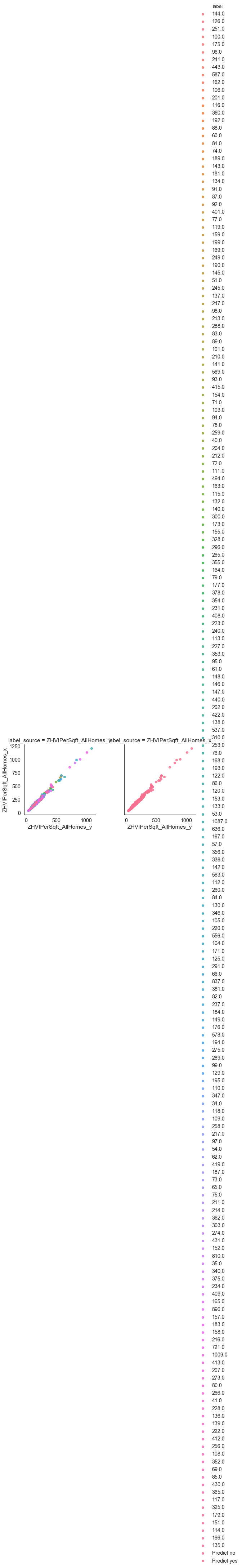
y_pred = gnb_model.predict(df_q5B_test[['ZHVIPerSqft_AllHomes_x']])
df_q5B_test['predicted_nb2'] = y_pred
/anaconda3/lib/python3.6/site-packages/ipykernel_launcher.py:2: SettingWithCopyWarning:
A value is trying to be set on a copy of a slice from a DataFrame.
Try using .loc[row_indexer,col_indexer] = value instead

See the caveats in the documentation: http://pandas.pydata.org/pandas-docs/stable/indexing.html#indexing-view-versus-copy
df_q5B_test
| RegionName | Year_x | ZHVIPerSqft_AllHomes_x | Year_y | ZHVIPerSqft_AllHomes_y | Dif | Label | predicted_nb | predicted_nb2 | |
|---|---|---|---|---|---|---|---|---|---|
| 778 | sacoyorkme | 2017 | 157.0 | 2015 | 144.0 | 13.0 | no | no | no |
| 114 | bristolhartfordct | 2017 | 128.0 | 2015 | 126.0 | 2.0 | no | no | no |
| 874 | stamfordfairfieldct | 2017 | 249.0 | 2015 | 251.0 | -2.0 | no | no | no |
| 75 | bethlehemnorthamptonpa | 2017 | 106.0 | 2015 | 100.0 | 6.0 | no | no | no |
| 568 | monroefairfieldct | 2017 | 173.0 | 2015 | 175.0 | -2.0 | no | no | no |
| 141 | cantonhaywoodnc | 2017 | 112.0 | 2015 | 96.0 | 16.0 | no | no | no |
| 2 | actonmiddlesexma | 2017 | 267.0 | 2015 | 241.0 | 26.0 | no | no | no |
| 362 | haikumauihi | 2017 | 485.0 | 2015 | 443.0 | 42.0 | no | no | no |
| 218 | daly_citysan_mateoca | 2017 | 693.0 | 2015 | 587.0 | 106.0 | yes | yes | yes |
| 546 | middletown_townshipbuckspa | 2017 | 169.0 | 2015 | 162.0 | 7.0 | no | no | no |
| 207 | cranstonprovidenceri | 2017 | 166.0 | 2015 | 144.0 | 22.0 | no | no | no |
| 685 | palmettomanateefl | 2017 | 128.0 | 2015 | 106.0 | 22.0 | no | no | no |
| 144 | carmelputnamny | 2017 | 213.0 | 2015 | 201.0 | 12.0 | no | no | no |
| 186 | colorado_springsel_pasoco | 2017 | 136.0 | 2015 | 116.0 | 20.0 | no | no | no |
| 326 | garden_groveorangeca | 2017 | 418.0 | 2015 | 360.0 | 58.0 | no | no | no |
| 152 | celebrationosceolafl | 2017 | 204.0 | 2015 | 192.0 | 12.0 | no | no | no |
| 355 | greergreenvillesc | 2017 | 99.0 | 2015 | 88.0 | 11.0 | no | no | no |
| 478 | little_fallsmorrisonmn | 2017 | 68.0 | 2015 | 60.0 | 8.0 | no | no | no |
| 403 | inmanspartanburgsc | 2017 | 92.0 | 2015 | 81.0 | 11.0 | no | no | no |
| 876 | statesvilleiredellnc | 2017 | 85.0 | 2015 | 74.0 | 11.0 | no | no | no |
| 507 | madisonnew_havenct | 2017 | 194.0 | 2015 | 189.0 | 5.0 | no | no | no |
| 699 | pembroke_pinesbrowardfl | 2017 | 168.0 | 2015 | 143.0 | 25.0 | no | no | no |
| 562 | minneapolishennepinmn | 2017 | 210.0 | 2015 | 181.0 | 29.0 | no | no | no |
| 551 | milford_townshipoaklandmi | 2017 | 148.0 | 2015 | 134.0 | 14.0 | no | no | no |
| 17 | altamonte_springsseminolefl | 2017 | 117.0 | 2015 | 91.0 | 26.0 | no | no | no |
| 189 | columbiaboonemo | 2017 | 93.0 | 2015 | 87.0 | 6.0 | no | no | no |
| 194 | concordcabarrusnc | 2017 | 104.0 | 2015 | 92.0 | 12.0 | no | no | no |
| 149 | castro_valleyalamedaca | 2017 | 467.0 | 2015 | 401.0 | 66.0 | no | no | no |
| 124 | buhltwin_fallsid | 2017 | 84.0 | 2015 | 77.0 | 7.0 | no | no | no |
| 96 | bonita_springsleefl | 2017 | 198.0 | 2015 | 181.0 | 17.0 | no | no | no |
| ... | ... | ... | ... | ... | ... | ... | ... | ... | ... |
| 53 | avonhartfordct | 2017 | 157.0 | 2015 | 157.0 | 0.0 | no | no | no |
| 487 | long_beachlos_angelesca | 2017 | 419.0 | 2015 | 365.0 | 54.0 | no | no | no |
| 411 | jasperduboisin | 2017 | 92.0 | 2015 | 86.0 | 6.0 | no | no | no |
| 821 | schaumburgcookil | 2017 | 171.0 | 2015 | 159.0 | 12.0 | no | no | no |
| 345 | grants_passjosephineor | 2017 | 162.0 | 2015 | 133.0 | 29.0 | no | no | no |
| 632 | northampton_townshipbuckspa | 2017 | 174.0 | 2015 | 171.0 | 3.0 | no | no | no |
| 738 | prospectjeffersonky | 2017 | 147.0 | 2015 | 136.0 | 11.0 | no | no | no |
| 319 | fremontdodgene | 2017 | 108.0 | 2015 | 97.0 | 11.0 | no | no | no |
| 210 | crestviewokaloosafl | 2017 | 91.0 | 2015 | 84.0 | 7.0 | no | no | no |
| 809 | sangerfresnoca | 2017 | 138.0 | 2015 | 117.0 | 21.0 | no | no | no |
| 350 | greensboroguilfordnc | 2017 | 87.0 | 2015 | 80.0 | 7.0 | no | no | no |
| 1019 | westboroughworcesterma | 2017 | 223.0 | 2015 | 201.0 | 22.0 | no | no | no |
| 302 | findlayhancockoh | 2017 | 85.0 | 2015 | 80.0 | 5.0 | no | no | no |
| 510 | malvernchesterpa | 2017 | 192.0 | 2015 | 183.0 | 9.0 | no | no | no |
| 1050 | woodburnmarionor | 2017 | 168.0 | 2015 | 126.0 | 42.0 | no | no | no |
| 978 | vestavia_hillsjeffersonal | 2017 | 151.0 | 2015 | 138.0 | 13.0 | no | no | no |
| 406 | island_parkfremontid | 2017 | 210.0 | 2015 | 192.0 | 18.0 | no | no | no |
| 588 | napervilledu_pageil | 2017 | 162.0 | 2015 | 158.0 | 4.0 | no | no | no |
| 825 | seasidemontereyca | 2017 | 393.0 | 2015 | 325.0 | 68.0 | no | no | no |
| 78 | biddefordyorkme | 2017 | 163.0 | 2015 | 149.0 | 14.0 | no | no | no |
| 70 | bellinghamwhatcomwa | 2017 | 215.0 | 2015 | 179.0 | 36.0 | no | no | no |
| 300 | fernandina_beachnassaufl | 2017 | 172.0 | 2015 | 151.0 | 21.0 | no | no | no |
| 785 | saint_georgewashingtonut | 2017 | 127.0 | 2015 | 114.0 | 13.0 | no | no | no |
| 964 | twin_fallstwin_fallsid | 2017 | 94.0 | 2015 | 85.0 | 9.0 | no | no | no |
| 58 | baltimorebaltimore_citymd | 2017 | 107.0 | 2015 | 99.0 | 8.0 | no | no | no |
| 306 | fontanasan_bernardinoca | 2017 | 219.0 | 2015 | 192.0 | 27.0 | no | no | no |
| 252 | east_greenwichkentri | 2017 | 192.0 | 2015 | 166.0 | 26.0 | no | no | no |
| 192 | columbusfranklinoh | 2017 | 93.0 | 2015 | 78.0 | 15.0 | no | no | no |
| 201 | coos_baycoosor | 2017 | 134.0 | 2015 | 118.0 | 16.0 | no | no | no |
| 1057 | worcesterworcesterma | 2017 | 150.0 | 2015 | 135.0 | 15.0 | no | no | no |
321 rows × 9 columns
invest = df_q5B_test.loc[df_q5B_test["predicted_nb2"]=="yes"]
invest.head()
| RegionName | Year_x | ZHVIPerSqft_AllHomes_x | Year_y | ZHVIPerSqft_AllHomes_y | Dif | Label | predicted_nb | predicted_nb2 | |
|---|---|---|---|---|---|---|---|---|---|
| 218 | daly_citysan_mateoca | 2017 | 693.0 | 2015 | 587.0 | 106.0 | yes | yes | yes |
| 795 | san_anselmomarinca | 2017 | 661.0 | 2015 | 569.0 | 92.0 | no | yes | yes |
| 757 | redondo_beachlos_angelesca | 2017 | 579.0 | 2015 | 494.0 | 85.0 | no | no | yes |
| 417 | kailuahonoluluhi | 2017 | 604.0 | 2015 | 537.0 | 67.0 | no | no | yes |
| 509 | malibulos_angelesca | 2017 | 1208.0 | 2015 | 1087.0 | 121.0 | yes | yes | yes |
final_data = invest.sort_values(by='ZHVIPerSqft_AllHomes_x')
final_data.to_csv("Output.csv",encoding='utf-8', index=False)
invest.head()
| RegionName | Year_x | ZHVIPerSqft_AllHomes_x | Year_y | ZHVIPerSqft_AllHomes_y | Dif | Label | predicted_nb | predicted_nb2 | |
|---|---|---|---|---|---|---|---|---|---|
| 218 | daly_citysan_mateoca | 2017 | 693.0 | 2015 | 587.0 | 106.0 | yes | yes | yes |
| 795 | san_anselmomarinca | 2017 | 661.0 | 2015 | 569.0 | 92.0 | no | yes | yes |
| 757 | redondo_beachlos_angelesca | 2017 | 579.0 | 2015 | 494.0 | 85.0 | no | no | yes |
| 417 | kailuahonoluluhi | 2017 | 604.0 | 2015 | 537.0 | 67.0 | no | no | yes |
| 509 | malibulos_angelesca | 2017 | 1208.0 | 2015 | 1087.0 | 121.0 | yes | yes | yes |
final_data.head()
| RegionName | Year_x | ZHVIPerSqft_AllHomes_x | Year_y | ZHVIPerSqft_AllHomes_y | Dif | Label | predicted_nb | predicted_nb2 | |
|---|---|---|---|---|---|---|---|---|---|
| 757 | redondo_beachlos_angelesca | 2017 | 579.0 | 2015 | 494.0 | 85.0 | no | no | yes |
| 417 | kailuahonoluluhi | 2017 | 604.0 | 2015 | 537.0 | 67.0 | no | no | yes |
| 392 | honoluluhonoluluhi | 2017 | 606.0 | 2015 | 556.0 | 50.0 | no | no | yes |
| 845 | solana_beachsan_diegoca | 2017 | 631.0 | 2015 | 578.0 | 53.0 | no | yes | yes |
| 795 | san_anselmomarinca | 2017 | 661.0 | 2015 | 569.0 | 92.0 | no | yes | yes |
Sample Data
sample_data = city_state_data.head(1000)
sample_data.to_csv("sample_data.csv",encoding='utf-8', index=False)